pacman::p_load(readxl, sf, tidyverse, tmap, sfdep, rvest, httr, jsonlite, onemapsgapi, ggpubr, olsrr, GWmodel, SpatialML, Metrics, ggplot2, plotly, spdep)1 Overview
1.1 Setting the Scene
Singapore’s Housing Development Board (HDB) flats are quite ubiquitous, being the most common housing type Singaporeans live in.
In recent months, questions about HDB affordability has been raised, which led to PM Lee’s assurance on affordability housing for all in Budget 2023. Yet, in the past year, more million dollar HDBswere resold.
So how could we understand and predict HDB resale prices? Are they due to the location and proximity to points of interest? Or are they due to the type and size of HDB? Could there also be unknown increased demand in certain geographical araes in Singapore that leads to many of these million dollar HDBs?
1.2 Tasks
We will work on constructing and comparing an OLS Multiple Linear Regression Model and Geographic Weighted Random Forest Model to predict 5-room HDB prices for the month of January and February 2023 in Singpaore.
The training data will consist of 5-room HDB resale data between January 2021 to December 2022.
2 Getting Started
2.1 Installing and Loading Packages
Next, pacman assists us by helping us load R packages that we require, sf, tidyverse and funModeling.
The following packages assists us to accomplish the following:
readxl assists us in importing
.xlsxaspatial data without having to convert to.csvsf helps to import, manage and process vector-based geospatial data in R
tidyverse which includes readr to import delimited text file, tidyr for tidying data and dplyr for wrangling data
tmap provides functions to allow us to plot high quality static or interactive maps using leaflet API
rvest, httr, jsonlite, onemapsgapi helps us to handle requests, convert json data and load datasets directly from onemap
ggpubr, ggplot2, plotly helps us with plotting the interactive and beautiful graphs
olsrr helps with Ordinary Least Squares Linear Regression
Gwmodel and SpatialML helps with the creation and prediction of Geographically Weighted Random Forest Machine Learning model
Metrics helps to calculate the RMSE (Root Means Squared Error) metrics for the prediction
spdep helps with calculation with nearest neighbours to provide data to calculate the Moran I’s statistics to determine clustering effects
2.2 Data Acquisition
The following datasets would be used to create the predictive models using conventional OLS and GWR methods for HDB Resale Prices.
| Dataset Type | Dataset Name | Remarks | Source |
|---|---|---|---|
| Geospatial | URA Master Plan 2019 Subzone Boundary | For visualisation purposes and extract Central Area | Prof Kam |
| Aspatial | HDB Resale Flat Prices | data.gov.sg | |
| Aspatial | HDB MUP/HIP Status | Manual Web Scraping | hdb.gov.sg |
| Aspatial | Shopping Malls | Manual web scraping | wikipedia.org : List of Shopping Malls in Singapore |
| Geospatial | Childcare | onemap.sg Themes | |
| Geospatial | Kindergartens | onemap.sg Themes | |
| Geospatial | Eldercare | onemap.sg Themes | |
| Geospatial | Foodcourt/Hawker | onemap.sg Themes | |
| Geospatial | Supermarket | onemap.sg | |
| Geospatial | Current and Future MRT/LRT Stations | Excludes Cross Region Line Punggol Branch | data.gov.sg |
| - | Future MRT Station (CRL Punggol Branch) | Manually merge into MRT/LRT Station Dataset | wikipedia.org : Elias MRT Stn wikipedia.org : Riveria MRT Stn |
| Geospatial | MRT/LRT Railway Line | Filter elevated sections of MRT line | data.gov.sg |
| Geospatial | Bus Stops | datamall.lta.gov.sg | |
| Geospatial | Parks | We consider the rail corridor, nature reserves and parks as parks as they are for leisure purposes. Also, we will prefer polygons of parks as we can calculate the actual proximity to the edges of the parks instead of to an arbitary point in the centre of the park. |
data.gov.sg |
| Geospatial | Primary Schools | Requires special handling | onemap.sg json |
| Aspatial | CHAS Clinics | Extracted using Excel from PDF | chas.sg |
2.3 Data Fields
The data fields we are looking to incorporate and work with in our predictive models includes:
Area of the unit
Floor level
Remaining lease
Age of the unit
Main Upgrading Program (MUP) completed
Extracted MUP and Home Improvment Programme (HIP) data from HDB website
For HDB units that has received HIP, their home value may be affected positively than a similar aged flat that has not received it
Flat Model (eg. DBSS/Standard/Premium)
Design Build Sell Scheme (DBSS) flats may call for a higher value than regular HDB flats as they are designed, build and sold by 3rd party developers although they are still HDB Flats. They are supposed to be better than premium flats
Premium flats which come with pre-installed fittings and furnishings over standard apartments which comes with none
Reference: https://www.teoalida.com/singapore/hdbflattypes/
Flat Multi-storey (Maisonette or Loft)
- Some homeowners may prefer multi-story HDBs over single-story ones
Proximity to CBD
Proximity to eldercare
Proximity to foodcourt/hawker centres
Proximity to MRT
Proximity to park
Proximity to good primary school
Proximity to shopping mall
Proximity to supermarket
Numbers of kindergartens within 350m
Numbers of childcare centres within 350m
Numbers of bus stop within 350m
Numbers of primary school within 1km
Proximity to Overhead MRT Line [noise concern]
- The closer a HDB unit is to the MRT track, the home value might be affected due to noise concerns. We measure the proximity of HDB units using its euclidean distance to the closest part of the MRT track if it is less than 300metres away.
Proximity to Overhead LRT Line (similar to MRT line)
Number of Future MRT stops within 800m (10min walk)
- Here, I want to explore how the resale values of HDBs could be affected by future MRT stations that are announced but not yet built. Home owners may be enticed to buy houses near future MRT lines in hopes that the house values will increase and also due to increased connectivity
Number of LRT Stops within 350m
- The metric is necessary as LRT serves as a feeder within the town and is typically used short-haul vs MRT which is between various towns. The 350m metric is derived from Bus Stops differentiates the weight between a LRT stop and MRT stop especially if the LRT stop is far away from the MRT stop in towns such as Sengkang, Punggol and Pasir Ris
3 Data Wrangling: Geospatial Data
There are two categories of datasets we will need for our analysis, these includes:
Datasets that has been downloaded - These files are already downloaded into a local location
Datasets that are retrieved over API - We need to obtain the datasets using API Calls
3.1 Importing / Retrieving / Obtaining Data
3.1.1 Retrieving Data from API Calls
There are some data that we need to retreive using API calls from onemap.sg. OneMap offers additional data from different government agencies through Themes. For R, the onemapsgapi package helps us with the API calls with onemap.sg servers to obtain the data we require.
Using onemapsgapi is pretty simple as shown below:
token <- "" # enter authentication token obtained from onemap
search_themes(token, "<searchterm>") %>% print(n=Inf)
tibble <- get_theme(token, "<queryname>")
sf <- st_as_sf(tibble, coords=c("Lng", "Lat"), crs=4326)search_themes() - Search for various thematic layers provided by onemap (eg. Parks). A tibble dataframe will be provided with more details of the layer, such as the
THEMENAME,QUERYNAME,ICON,CATEGORYandTHEME_OWNERget_theme() - Using the desired theme’s
QUERYNAMEobtained from search_themes(), we can obtain the thematic data in a tibble dataframe. We will need to use st_as_sf to specify theLat,Lngand crs to obtain it as a sf dataframe.
Listed below are a list of layers we need to obtain:
Childcare
Kindergartens
Eldercare
Foodcourt/Hawker Centres
In the code block below, we will assume to have used search_themes() to pick the specific themes we want, to load them. The justification will be listed below.
Childcare
childcare_tibble <- get_theme(token, "childcare")
childcare_sf <- st_as_sf(childcare_tibble, coords=c("Lng", "Lat"), crs=4326)Kindergartens
kindergartens_tibble <- get_theme(token, "kindergartens")
kindergartens_sf <- st_as_sf(kindergartens_tibble, coords=c("Lng", "Lat"), crs=4326)Eldercare
eldercare_tibble <- get_theme(token, "eldercare")
eldercare_sf <- st_as_sf(eldercare_tibble, coords=c("Lng", "Lat"), crs=4326)Foodcourt/Hawker Centre
hawker_tibble <- get_theme(token, "hawkercentre_new")
hawker_sf <- st_as_sf(hawker_tibble, coords=c("Lng", "Lat"), crs=4326)write_rds(childcare_sf, "Take-Home_Ex03/rds/childcare_sf.rds")
write_rds(kindergartens_sf, "Take-Home_Ex03/rds/kindergartens_sf.rds")
write_rds(eldercare_sf, "Take-Home_Ex03/rds/eldercare_sf.rds")
write_rds(hawker_sf, "Take-Home_Ex03/rds/hawker_sf.rds")3.1.2 Obtaining Schools Data
Obtaining school data from OneMap is a bit tricky, it was not available through OneMap themes or a download link through the OneMap website. However, through clicking through the Query Schools function on the map using using ‘Inspect Element’, we could see that a GET request is called to obtain the map data as json (as seen in the screenshot below):
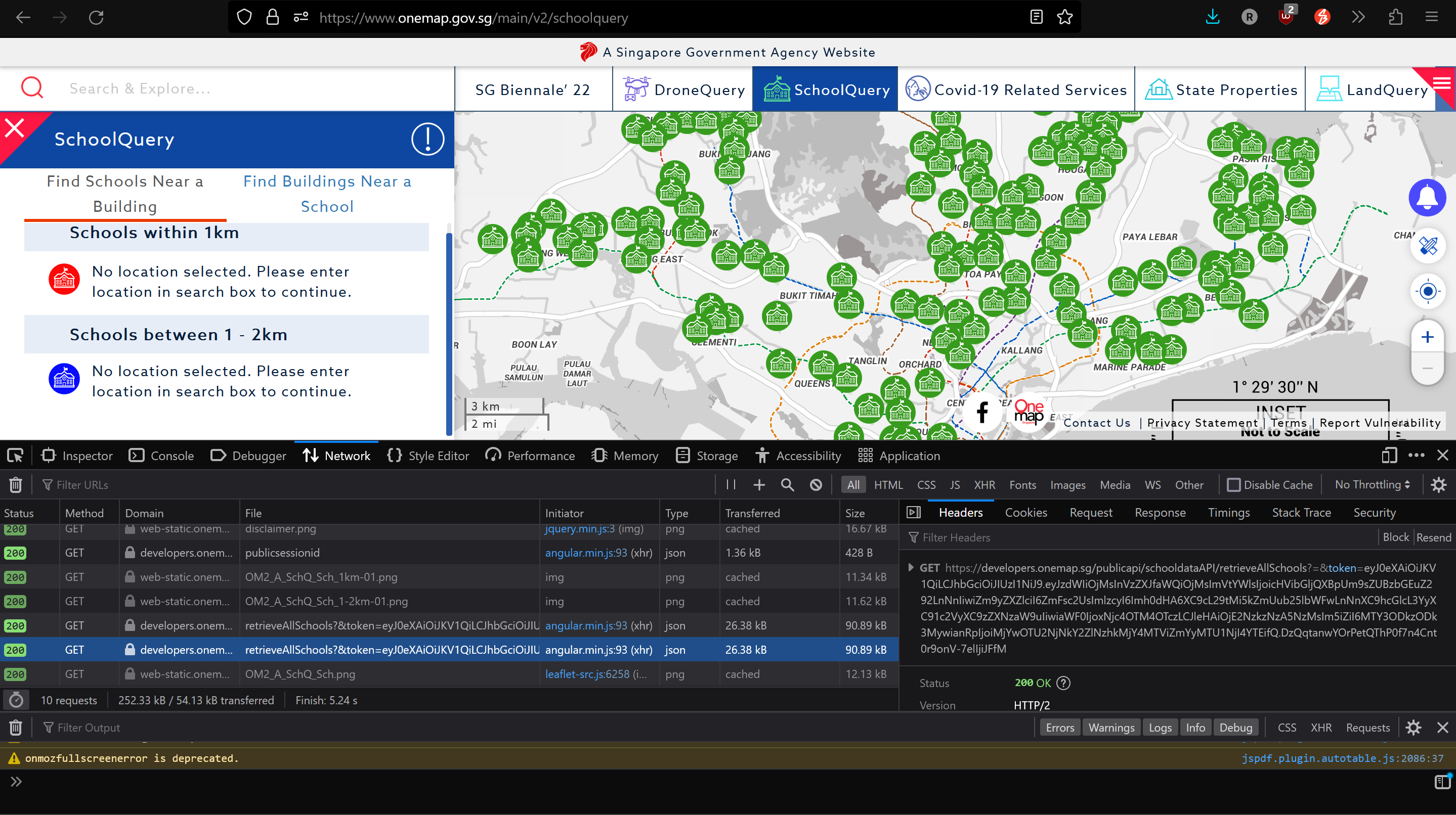
By opening the link, we could see that it is an undocumented public API that OneMap uses to retrieve map data regarding Primary Schools. The results are in json as shown below:
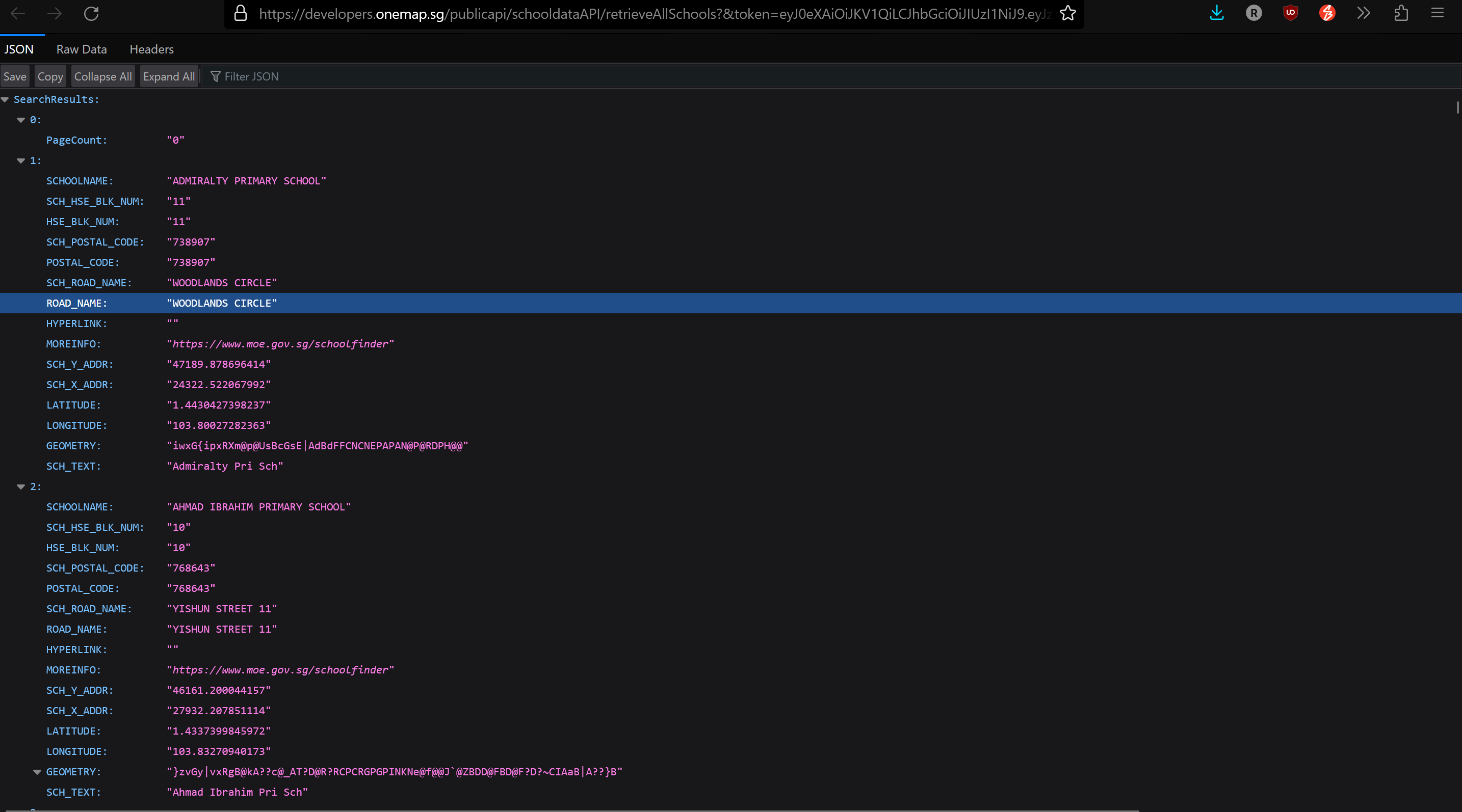
The data has been downloaded and will be processed into tibble format using json_lite fromJSON() which will import the JSON file and convert it into tibble dataframe.
schools_tibble <- fromJSON("Take-Home_Ex03/geospatial/retrieveAllSchools.json")[["SearchResults"]]
glimpse(schools_tibble)Rows: 182
Columns: 16
$ PageCount <chr> "0", NA, NA, NA, NA, NA, NA, NA, NA, NA, NA, NA, NA, N…
$ SCHOOLNAME <chr> NA, "ADMIRALTY PRIMARY SCHOOL", "AHMAD IBRAHIM PRIMARY…
$ SCH_HSE_BLK_NUM <chr> NA, "11", "10", "100", "2A", "31", "19", "20", "16", "…
$ HSE_BLK_NUM <chr> NA, "11", "10", "100", "2A", "31", "19", "20", "16", "…
$ SCH_POSTAL_CODE <chr> NA, "738907", "768643", "579646", "159016", "544969", …
$ POSTAL_CODE <chr> NA, "738907", "768643", "579646", "159016", "544969", …
$ SCH_ROAD_NAME <chr> NA, "WOODLANDS CIRCLE", "YISHUN STREET 11", "BRIGHT HI…
$ ROAD_NAME <chr> NA, "WOODLANDS CIRCLE", "YISHUN STREET 11", "BRIGHT HI…
$ HYPERLINK <chr> NA, "", "", "", "", "", "", "", "", "", "", "", "", ""…
$ MOREINFO <chr> NA, "https://www.moe.gov.sg/schoolfinder", "https://ww…
$ SCH_Y_ADDR <chr> NA, "47189.878696414", "46161.200044157", "38079.99126…
$ SCH_X_ADDR <chr> NA, "24322.522067992", "27932.207851114", "27956.93877…
$ LATITUDE <chr> NA, "1.4430427398237", "1.4337399845972", "1.360656435…
$ LONGITUDE <chr> NA, "103.80027282363", "103.83270940173", "103.8329316…
$ GEOMETRY <chr> NA, "iwxG{ipxRXm@p@UsBcGsE|AdBdFFCNCNEPAPAN@P@RDPH@@",…
$ SCH_TEXT <chr> NA, "Admiralty Pri Sch", "Ahmad Ibrahim Pri Sch", "Ai …As we can see the want to exclude the column PageCount and the first row as it is not relavant to our dataset. The code chunk below will perform the above for us:
schools_tibble <- select(schools_tibble,-"PageCount")
schools_tibble <- schools_tibble[-1,]Next, we will convert the tibble dataframe to sf dataframe. Since X and Y coordinates are provided for us (SVY21) in the columns SCH_Y_ADDR and SCH_X_ADDR, we will use them instead of the Lng and Lat as SVY21 (Projected Coordinate System) will allow us to perform our analysis directly.
schools_sf_3414 <- st_as_sf(schools_tibble, coords=c("SCH_X_ADDR", "SCH_Y_ADDR"), crs=3414)Now, we will save the data imported as RDS file format (R Data Serialisation).
write_rds(schools_sf_3414, "Take-Home_Ex03/rds/schools_sf_3414.rds")3.1.3 Importing Geospatial Data
Master Plan Subzone 2019
mpsz = st_read(dsn = "Take-Home_Ex03/geospatial", layer="MPSZ-2019")Reading layer `MPSZ-2019' from data source
`C:\renjie-teo\IS415-GAA\exercises\Take-Home_Ex03\geospatial'
using driver `ESRI Shapefile'
Simple feature collection with 332 features and 6 fields
Geometry type: MULTIPOLYGON
Dimension: XY
Bounding box: xmin: 103.6057 ymin: 1.158699 xmax: 104.0885 ymax: 1.470775
Geodetic CRS: WGS 84Current and Future MRT/LRT Stations
geo_mrt_lrt_stn = st_read(dsn = "Take-Home_Ex03/geospatial/master-plan-2019-rail-station-layer-kml.kml")Reading layer `G_MP19_RAIL_STN_PL' from data source
`C:\renjie-teo\IS415-GAA\exercises\Take-Home_Ex03\geospatial\master-plan-2019-rail-station-layer-kml.kml'
using driver `KML'
Simple feature collection with 257 features and 2 fields
Geometry type: MULTIPOLYGON
Dimension: XY, XYZ
Bounding box: xmin: 103.6363 ymin: 1.251433 xmax: 104.0051 ymax: 1.449548
z_range: zmin: 0 zmax: 0
Geodetic CRS: WGS 84MRT/LRT Railway Line
geo_railway_line = st_read(dsn = "Take-Home_Ex03/geospatial/rail-line.kml")Reading layer `G_MP19_RAIL_LINE_LI' from data source
`C:\renjie-teo\IS415-GAA\exercises\Take-Home_Ex03\geospatial\rail-line.kml'
using driver `KML'
Simple feature collection with 1366 features and 2 fields
Geometry type: MULTILINESTRING
Dimension: XY, XYZ
Bounding box: xmin: 103.6352 ymin: 1.251689 xmax: 104.0201 ymax: 1.45265
z_range: zmin: 0 zmax: 0
Geodetic CRS: WGS 84Bus Stops
geo_bus_stop = st_read(dsn = "Take-Home_Ex03/geospatial", layer="BusStop")Reading layer `BusStop' from data source
`C:\renjie-teo\IS415-GAA\exercises\Take-Home_Ex03\geospatial'
using driver `ESRI Shapefile'
Simple feature collection with 5159 features and 3 fields
Geometry type: POINT
Dimension: XY
Bounding box: xmin: 3970.122 ymin: 26482.1 xmax: 48284.56 ymax: 52983.82
Projected CRS: SVY21Parks
geo_parks = st_read(dsn = "Take-Home_Ex03/geospatial/nparks-parks-and-nature-reserves-kml.kml")Reading layer `NParks_Parks' from data source
`C:\renjie-teo\IS415-GAA\exercises\Take-Home_Ex03\geospatial\nparks-parks-and-nature-reserves-kml.kml'
using driver `KML'
Simple feature collection with 421 features and 2 fields
Geometry type: MULTIPOLYGON
Dimension: XYZ
Bounding box: xmin: 103.6925 ymin: 1.2115 xmax: 104.0544 ymax: 1.46419
z_range: zmin: 0 zmax: 0
Geodetic CRS: WGS 84Supermarket
geo_supermarkets = st_read(dsn = "Take-Home_Ex03/geospatial", layer="Supermarkets")Reading layer `Supermarkets' from data source
`C:\renjie-teo\IS415-GAA\exercises\Take-Home_Ex03\geospatial'
using driver `ESRI Shapefile'
Simple feature collection with 526 features and 8 fields
Geometry type: POINT
Dimension: XY
Bounding box: xmin: 4901.188 ymin: 25529.08 xmax: 46948.22 ymax: 49233.6
Projected CRS: SVY21geo_schools <- read_rds("Take-Home_Ex03/rds/schools_sf_3414.rds")
geo_childcare <- read_rds("Take-Home_Ex03/rds/childcare_sf.rds")
geo_eldercare <- read_rds("Take-Home_Ex03/rds/eldercare_sf.rds")
geo_hawker <- read_rds("Take-Home_Ex03/rds/hawker_sf.rds")
geo_kindergartens <- read_rds("Take-Home_Ex03/rds/kindergartens_sf.rds")3.2 Transforming Coordinate Systems
For datasets in WGS84 Geodetic Coordinate System, we need to convert them to SVY21 Projected Coordinate System to perform our analysis. Inferring form the information above, we will use the code chunk below to confirm all of them.
We use st_zm() on the kml datasets to remove the Z dimensions which will cause issues with analysis later as XY and XYZ data do not work well with one another.
mpsz <- st_transform(mpsz,3414)
geo_mrt_lrt_stn <- st_transform(st_zm(geo_mrt_lrt_stn),3414)
geo_railway_line <- st_transform(st_zm(geo_railway_line),3414)
geo_parks <- st_transform(st_zm(geo_parks),3414)
geo_supermarkets <- st_transform(geo_supermarkets,3414)
geo_childcare <- st_transform(geo_childcare,3414)
geo_eldercare <- st_transform(geo_eldercare,3414)
geo_hawker <- st_transform(geo_hawker,3414)
geo_kindergartens <- st_transform(geo_kindergartens,3414)Bus Stop
st_crs(geo_bus_stop)Coordinate Reference System:
User input: SVY21
wkt:
PROJCRS["SVY21",
BASEGEOGCRS["WGS 84",
DATUM["World Geodetic System 1984",
ELLIPSOID["WGS 84",6378137,298.257223563,
LENGTHUNIT["metre",1]],
ID["EPSG",6326]],
PRIMEM["Greenwich",0,
ANGLEUNIT["Degree",0.0174532925199433]]],
CONVERSION["unnamed",
METHOD["Transverse Mercator",
ID["EPSG",9807]],
PARAMETER["Latitude of natural origin",1.36666666666667,
ANGLEUNIT["Degree",0.0174532925199433],
ID["EPSG",8801]],
PARAMETER["Longitude of natural origin",103.833333333333,
ANGLEUNIT["Degree",0.0174532925199433],
ID["EPSG",8802]],
PARAMETER["Scale factor at natural origin",1,
SCALEUNIT["unity",1],
ID["EPSG",8805]],
PARAMETER["False easting",28001.642,
LENGTHUNIT["metre",1],
ID["EPSG",8806]],
PARAMETER["False northing",38744.572,
LENGTHUNIT["metre",1],
ID["EPSG",8807]]],
CS[Cartesian,2],
AXIS["(E)",east,
ORDER[1],
LENGTHUNIT["metre",1,
ID["EPSG",9001]]],
AXIS["(N)",north,
ORDER[2],
LENGTHUNIT["metre",1,
ID["EPSG",9001]]]]Oh, the CRS was not set properly and reflected as EPSG:9001
geo_bus_stop <- st_set_crs(geo_bus_stop, 3414)
st_crs(geo_bus_stop)Coordinate Reference System:
User input: EPSG:3414
wkt:
PROJCRS["SVY21 / Singapore TM",
BASEGEOGCRS["SVY21",
DATUM["SVY21",
ELLIPSOID["WGS 84",6378137,298.257223563,
LENGTHUNIT["metre",1]]],
PRIMEM["Greenwich",0,
ANGLEUNIT["degree",0.0174532925199433]],
ID["EPSG",4757]],
CONVERSION["Singapore Transverse Mercator",
METHOD["Transverse Mercator",
ID["EPSG",9807]],
PARAMETER["Latitude of natural origin",1.36666666666667,
ANGLEUNIT["degree",0.0174532925199433],
ID["EPSG",8801]],
PARAMETER["Longitude of natural origin",103.833333333333,
ANGLEUNIT["degree",0.0174532925199433],
ID["EPSG",8802]],
PARAMETER["Scale factor at natural origin",1,
SCALEUNIT["unity",1],
ID["EPSG",8805]],
PARAMETER["False easting",28001.642,
LENGTHUNIT["metre",1],
ID["EPSG",8806]],
PARAMETER["False northing",38744.572,
LENGTHUNIT["metre",1],
ID["EPSG",8807]]],
CS[Cartesian,2],
AXIS["northing (N)",north,
ORDER[1],
LENGTHUNIT["metre",1]],
AXIS["easting (E)",east,
ORDER[2],
LENGTHUNIT["metre",1]],
USAGE[
SCOPE["Cadastre, engineering survey, topographic mapping."],
AREA["Singapore - onshore and offshore."],
BBOX[1.13,103.59,1.47,104.07]],
ID["EPSG",3414]]Done!
Master Plan Subzone 2019
mpszSimple feature collection with 332 features and 6 fields
Geometry type: MULTIPOLYGON
Dimension: XY
Bounding box: xmin: 2667.538 ymin: 15748.72 xmax: 56396.44 ymax: 50256.33
Projected CRS: SVY21 / Singapore TM
First 10 features:
SUBZONE_N SUBZONE_C PLN_AREA_N PLN_AREA_C REGION_N
1 MARINA EAST MESZ01 MARINA EAST ME CENTRAL REGION
2 INSTITUTION HILL RVSZ05 RIVER VALLEY RV CENTRAL REGION
3 ROBERTSON QUAY SRSZ01 SINGAPORE RIVER SR CENTRAL REGION
4 JURONG ISLAND AND BUKOM WISZ01 WESTERN ISLANDS WI WEST REGION
5 FORT CANNING MUSZ02 MUSEUM MU CENTRAL REGION
6 MARINA EAST (MP) MPSZ05 MARINE PARADE MP CENTRAL REGION
7 SUDONG WISZ03 WESTERN ISLANDS WI WEST REGION
8 SEMAKAU WISZ02 WESTERN ISLANDS WI WEST REGION
9 SOUTHERN GROUP SISZ02 SOUTHERN ISLANDS SI CENTRAL REGION
10 SENTOSA SISZ01 SOUTHERN ISLANDS SI CENTRAL REGION
REGION_C geometry
1 CR MULTIPOLYGON (((33222.98 29...
2 CR MULTIPOLYGON (((28481.45 30...
3 CR MULTIPOLYGON (((28087.34 30...
4 WR MULTIPOLYGON (((14557.7 304...
5 CR MULTIPOLYGON (((29542.53 31...
6 CR MULTIPOLYGON (((35279.55 30...
7 WR MULTIPOLYGON (((15772.59 21...
8 WR MULTIPOLYGON (((19843.41 21...
9 CR MULTIPOLYGON (((30870.53 22...
10 CR MULTIPOLYGON (((26879.04 26...Current and Future MRT/LRT Stations
geo_mrt_lrt_stnSimple feature collection with 257 features and 2 fields
Geometry type: MULTIPOLYGON
Dimension: XY
Bounding box: xmin: 6071.311 ymin: 26002.6 xmax: 47112.64 ymax: 47909.19
Projected CRS: SVY21 / Singapore TM
First 10 features:
Name
1 kml_1
2 kml_2
3 kml_3
4 kml_4
5 kml_5
6 kml_6
7 kml_7
8 kml_8
9 kml_9
10 kml_10
Description
1 <center><table><tr><th colspan='2' align='center'><em>Attributes</em></th></tr><tr bgcolor="#E3E3F3"> <th>GRND_LEVEL</th> <td>ABOVEGROUND</td> </tr><tr bgcolor=""> <th>RAIL_TYPE</th> <td>LRT</td> </tr><tr bgcolor="#E3E3F3"> <th>NAME</th> <td>PUNGGOL CENTRAL</td> </tr><tr bgcolor=""> <th>INC_CRC</th> <td>5ED154CD47409638</td> </tr><tr bgcolor="#E3E3F3"> <th>FMEL_UPD_D</th> <td>20191209180316</td> </tr></table></center>
2 <center><table><tr><th colspan='2' align='center'><em>Attributes</em></th></tr><tr bgcolor="#E3E3F3"> <th>GRND_LEVEL</th> <td>ABOVEGROUND</td> </tr><tr bgcolor=""> <th>RAIL_TYPE</th> <td>LRT</td> </tr><tr bgcolor="#E3E3F3"> <th>NAME</th> <td>KANGKAR</td> </tr><tr bgcolor=""> <th>INC_CRC</th> <td>B4ACD980B1469EC8</td> </tr><tr bgcolor="#E3E3F3"> <th>FMEL_UPD_D</th> <td>20191209180316</td> </tr></table></center>
3 <center><table><tr><th colspan='2' align='center'><em>Attributes</em></th></tr><tr bgcolor="#E3E3F3"> <th>GRND_LEVEL</th> <td>UNDERGROUND</td> </tr><tr bgcolor=""> <th>RAIL_TYPE</th> <td>MRT</td> </tr><tr bgcolor="#E3E3F3"> <th>NAME</th> <td>SENGKANG</td> </tr><tr bgcolor=""> <th>INC_CRC</th> <td>632967D234F4FBC1</td> </tr><tr bgcolor="#E3E3F3"> <th>FMEL_UPD_D</th> <td>20191209180316</td> </tr></table></center>
4 <center><table><tr><th colspan='2' align='center'><em>Attributes</em></th></tr><tr bgcolor="#E3E3F3"> <th>GRND_LEVEL</th> <td>ABOVEGROUND</td> </tr><tr bgcolor=""> <th>RAIL_TYPE</th> <td>LRT</td> </tr><tr bgcolor="#E3E3F3"> <th>NAME</th> <td>PUNGGOL POINT</td> </tr><tr bgcolor=""> <th>INC_CRC</th> <td>933DB538DAED1131</td> </tr><tr bgcolor="#E3E3F3"> <th>FMEL_UPD_D</th> <td>20191209180316</td> </tr></table></center>
5 <center><table><tr><th colspan='2' align='center'><em>Attributes</em></th></tr><tr bgcolor="#E3E3F3"> <th>GRND_LEVEL</th> <td>ABOVEGROUND</td> </tr><tr bgcolor=""> <th>RAIL_TYPE</th> <td>LRT</td> </tr><tr bgcolor="#E3E3F3"> <th>NAME</th> <td>TONGKANG</td> </tr><tr bgcolor=""> <th>INC_CRC</th> <td>85E14C78B24F5DA1</td> </tr><tr bgcolor="#E3E3F3"> <th>FMEL_UPD_D</th> <td>20191209180316</td> </tr></table></center>
6 <center><table><tr><th colspan='2' align='center'><em>Attributes</em></th></tr><tr bgcolor="#E3E3F3"> <th>GRND_LEVEL</th> <td>ABOVEGROUND</td> </tr><tr bgcolor=""> <th>RAIL_TYPE</th> <td>LRT</td> </tr><tr bgcolor="#E3E3F3"> <th>NAME</th> <td>THANGGAM</td> </tr><tr bgcolor=""> <th>INC_CRC</th> <td>37F224D49C361EFD</td> </tr><tr bgcolor="#E3E3F3"> <th>FMEL_UPD_D</th> <td>20191209180316</td> </tr></table></center>
7 <center><table><tr><th colspan='2' align='center'><em>Attributes</em></th></tr><tr bgcolor="#E3E3F3"> <th>GRND_LEVEL</th> <td>ABOVEGROUND</td> </tr><tr bgcolor=""> <th>RAIL_TYPE</th> <td>LRT</td> </tr><tr bgcolor="#E3E3F3"> <th>NAME</th> <td>CORAL EDGE</td> </tr><tr bgcolor=""> <th>INC_CRC</th> <td>A49DD0F3F8F5B582</td> </tr><tr bgcolor="#E3E3F3"> <th>FMEL_UPD_D</th> <td>20191209180316</td> </tr></table></center>
8 <center><table><tr><th colspan='2' align='center'><em>Attributes</em></th></tr><tr bgcolor="#E3E3F3"> <th>GRND_LEVEL</th> <td>UNDERGROUND</td> </tr><tr bgcolor=""> <th>RAIL_TYPE</th> <td>MRT</td> </tr><tr bgcolor="#E3E3F3"> <th>NAME</th> <td>SERANGOON INTERCHANGE</td> </tr><tr bgcolor=""> <th>INC_CRC</th> <td>10AD56727C54F2E3</td> </tr><tr bgcolor="#E3E3F3"> <th>FMEL_UPD_D</th> <td>20191209180316</td> </tr></table></center>
9 <center><table><tr><th colspan='2' align='center'><em>Attributes</em></th></tr><tr bgcolor="#E3E3F3"> <th>GRND_LEVEL</th> <td>ABOVEGROUND</td> </tr><tr bgcolor=""> <th>RAIL_TYPE</th> <td>LRT</td> </tr><tr bgcolor="#E3E3F3"> <th>NAME</th> <td>RENJONG</td> </tr><tr bgcolor=""> <th>INC_CRC</th> <td>EA8A90EE63391CC1</td> </tr><tr bgcolor="#E3E3F3"> <th>FMEL_UPD_D</th> <td>20191209180316</td> </tr></table></center>
10 <center><table><tr><th colspan='2' align='center'><em>Attributes</em></th></tr><tr bgcolor="#E3E3F3"> <th>GRND_LEVEL</th> <td>UNDERGROUND</td> </tr><tr bgcolor=""> <th>RAIL_TYPE</th> <td>MRT</td> </tr><tr bgcolor="#E3E3F3"> <th>NAME</th> <td>SERANGOON INTERCHANGE</td> </tr><tr bgcolor=""> <th>INC_CRC</th> <td>E7D5531A772135B5</td> </tr><tr bgcolor="#E3E3F3"> <th>FMEL_UPD_D</th> <td>20191209180316</td> </tr></table></center>
geometry
1 MULTIPOLYGON (((35733.24 43...
2 MULTIPOLYGON (((35663.22 40...
3 MULTIPOLYGON (((34864.22 41...
4 MULTIPOLYGON (((36122.13 44...
5 MULTIPOLYGON (((33877.4 412...
6 MULTIPOLYGON (((32716.21 42...
7 MULTIPOLYGON (((36786.93 41...
8 MULTIPOLYGON (((32441.88 36...
9 MULTIPOLYGON (((34382.66 40...
10 MULTIPOLYGON (((32244.31 36...MRT/LRT Railway Line
geo_railway_lineSimple feature collection with 1366 features and 2 fields
Geometry type: MULTILINESTRING
Dimension: XY
Bounding box: xmin: 5950.856 ymin: 26030.91 xmax: 48791.81 ymax: 48252.23
Projected CRS: SVY21 / Singapore TM
First 10 features:
Name
1 kml_1
2 kml_2
3 kml_3
4 kml_4
5 kml_5
6 kml_6
7 kml_7
8 kml_8
9 kml_9
10 kml_10
Description
1 <center><table><tr><th colspan='2' align='center'><em>Attributes</em></th></tr><tr bgcolor="#E3E3F3"> <th>GRND_LEVEL</th> <td>ABOVEGROUND</td> </tr><tr bgcolor=""> <th>RAIL_TYPE</th> <td>MRT</td> </tr><tr bgcolor="#E3E3F3"> <th>INC_CRC</th> <td>19247B0E0E15AF87</td> </tr><tr bgcolor=""> <th>FMEL_UPD_D</th> <td>20191209172332</td> </tr></table></center>
2 <center><table><tr><th colspan='2' align='center'><em>Attributes</em></th></tr><tr bgcolor="#E3E3F3"> <th>GRND_LEVEL</th> <td>UNDERGROUND</td> </tr><tr bgcolor=""> <th>RAIL_TYPE</th> <td>MRT</td> </tr><tr bgcolor="#E3E3F3"> <th>INC_CRC</th> <td>66F16A9502E84AAB</td> </tr><tr bgcolor=""> <th>FMEL_UPD_D</th> <td>20191209172332</td> </tr></table></center>
3 <center><table><tr><th colspan='2' align='center'><em>Attributes</em></th></tr><tr bgcolor="#E3E3F3"> <th>GRND_LEVEL</th> <td>UNDERGROUND</td> </tr><tr bgcolor=""> <th>RAIL_TYPE</th> <td>MRT</td> </tr><tr bgcolor="#E3E3F3"> <th>INC_CRC</th> <td>33321452CB2EF3CA</td> </tr><tr bgcolor=""> <th>FMEL_UPD_D</th> <td>20191209172332</td> </tr></table></center>
4 <center><table><tr><th colspan='2' align='center'><em>Attributes</em></th></tr><tr bgcolor="#E3E3F3"> <th>GRND_LEVEL</th> <td>ABOVEGROUND</td> </tr><tr bgcolor=""> <th>RAIL_TYPE</th> <td>MRT</td> </tr><tr bgcolor="#E3E3F3"> <th>INC_CRC</th> <td>4E3C7F23EFA39E37</td> </tr><tr bgcolor=""> <th>FMEL_UPD_D</th> <td>20191209172332</td> </tr></table></center>
5 <center><table><tr><th colspan='2' align='center'><em>Attributes</em></th></tr><tr bgcolor="#E3E3F3"> <th>GRND_LEVEL</th> <td>ABOVEGROUND</td> </tr><tr bgcolor=""> <th>RAIL_TYPE</th> <td>MRT</td> </tr><tr bgcolor="#E3E3F3"> <th>INC_CRC</th> <td>F49903A9C3D88B3E</td> </tr><tr bgcolor=""> <th>FMEL_UPD_D</th> <td>20191209172332</td> </tr></table></center>
6 <center><table><tr><th colspan='2' align='center'><em>Attributes</em></th></tr><tr bgcolor="#E3E3F3"> <th>GRND_LEVEL</th> <td>ABOVEGROUND</td> </tr><tr bgcolor=""> <th>RAIL_TYPE</th> <td>MRT</td> </tr><tr bgcolor="#E3E3F3"> <th>INC_CRC</th> <td>68F669414248D951</td> </tr><tr bgcolor=""> <th>FMEL_UPD_D</th> <td>20191209172332</td> </tr></table></center>
7 <center><table><tr><th colspan='2' align='center'><em>Attributes</em></th></tr><tr bgcolor="#E3E3F3"> <th>GRND_LEVEL</th> <td>ABOVEGROUND</td> </tr><tr bgcolor=""> <th>RAIL_TYPE</th> <td>MRT</td> </tr><tr bgcolor="#E3E3F3"> <th>INC_CRC</th> <td>DCF940C0F51904A8</td> </tr><tr bgcolor=""> <th>FMEL_UPD_D</th> <td>20191209172332</td> </tr></table></center>
8 <center><table><tr><th colspan='2' align='center'><em>Attributes</em></th></tr><tr bgcolor="#E3E3F3"> <th>GRND_LEVEL</th> <td>UNDERGROUND</td> </tr><tr bgcolor=""> <th>RAIL_TYPE</th> <td>MRT</td> </tr><tr bgcolor="#E3E3F3"> <th>INC_CRC</th> <td>F9EF3225D6023E91</td> </tr><tr bgcolor=""> <th>FMEL_UPD_D</th> <td>20191209172332</td> </tr></table></center>
9 <center><table><tr><th colspan='2' align='center'><em>Attributes</em></th></tr><tr bgcolor="#E3E3F3"> <th>GRND_LEVEL</th> <td>UNDERGROUND</td> </tr><tr bgcolor=""> <th>RAIL_TYPE</th> <td>MRT</td> </tr><tr bgcolor="#E3E3F3"> <th>INC_CRC</th> <td>CFEF0AB02AC53C6F</td> </tr><tr bgcolor=""> <th>FMEL_UPD_D</th> <td>20191209172332</td> </tr></table></center>
10 <center><table><tr><th colspan='2' align='center'><em>Attributes</em></th></tr><tr bgcolor="#E3E3F3"> <th>GRND_LEVEL</th> <td>UNDERGROUND</td> </tr><tr bgcolor=""> <th>RAIL_TYPE</th> <td>MRT</td> </tr><tr bgcolor="#E3E3F3"> <th>INC_CRC</th> <td>636B424340907BC5</td> </tr><tr bgcolor=""> <th>FMEL_UPD_D</th> <td>20191209172332</td> </tr></table></center>
geometry
1 MULTILINESTRING ((20846.61 ...
2 MULTILINESTRING ((32943 373...
3 MULTILINESTRING ((32810.33 ...
4 MULTILINESTRING ((28086.31 ...
5 MULTILINESTRING ((28080.58 ...
6 MULTILINESTRING ((27410.68 ...
7 MULTILINESTRING ((27414.85 ...
8 MULTILINESTRING ((31030.73 ...
9 MULTILINESTRING ((30543.79 ...
10 MULTILINESTRING ((30410.42 ...Parks
geo_parksSimple feature collection with 421 features and 2 fields
Geometry type: MULTIPOLYGON
Dimension: XY
Bounding box: xmin: 12328.7 ymin: 21587.04 xmax: 52607.43 ymax: 49528.21
Projected CRS: SVY21 / Singapore TM
First 10 features:
Name
1 JANGGUS GARDEN
2 JLN LIMAU MANIS PG
3 GARDEN VIEW PG
4 THOMSON GREEN PG
5 JLN RIANG PG
6 MEI HWAN CRESCENT PG
7 FULTON AVE PG
8 MIMOSA TERRACE PG
9 JLN GENENG INTERIM PK
10 LENTOR WALK PG
Description
1 <html xmlns:fo="http://www.w3.org/1999/XSL/Format" xmlns:msxsl="urn:schemas-microsoft-com:xslt"> <head> <META http-equiv="Content-Type" content="text/html"> <meta http-equiv="content-type" content="text/html; charset=UTF-8"> </head> <body style="margin:0px 0px 0px 0px;overflow:auto;background:#FFFFFF;"> <table style="font-family:Arial,Verdana,Times;font-size:12px;text-align:left;width:100%;border-collapse:collapse;padding:3px 3px 3px 3px"> <tr style="text-align:center;font-weight:bold;background:#9CBCE2"> <td>JANGGUS GARDEN</td> </tr> <tr> <td> <table style="font-family:Arial,Verdana,Times;font-size:12px;text-align:left;width:100%;border-spacing:0px; padding:3px 3px 3px 3px"> <tr> <td>NAME</td> <td>JANGGUS GARDEN</td> </tr> <tr bgcolor="#D4E4F3"> <td>N_RESERVE</td> <td>0</td> </tr> <tr> <td>L_CODE</td> <td>NS524</td> </tr> </table> </td> </tr> </table> </body><script type="text/javascript"> function changeImage(attElement, nameElement) { document.getElementById('imageAttachment').src = attElement; document.getElementById('imageName').innerHTML = nameElement;} </script></html>
2 <html xmlns:fo="http://www.w3.org/1999/XSL/Format" xmlns:msxsl="urn:schemas-microsoft-com:xslt"> <head> <META http-equiv="Content-Type" content="text/html"> <meta http-equiv="content-type" content="text/html; charset=UTF-8"> </head> <body style="margin:0px 0px 0px 0px;overflow:auto;background:#FFFFFF;"> <table style="font-family:Arial,Verdana,Times;font-size:12px;text-align:left;width:100%;border-collapse:collapse;padding:3px 3px 3px 3px"> <tr style="text-align:center;font-weight:bold;background:#9CBCE2"> <td>JLN LIMAU MANIS PG</td> </tr> <tr> <td> <table style="font-family:Arial,Verdana,Times;font-size:12px;text-align:left;width:100%;border-spacing:0px; padding:3px 3px 3px 3px"> <tr> <td>NAME</td> <td>JLN LIMAU MANIS PG</td> </tr> <tr bgcolor="#D4E4F3"> <td>N_RESERVE</td> <td>0</td> </tr> <tr> <td>L_CODE</td> <td>EC508</td> </tr> </table> </td> </tr> </table> </body><script type="text/javascript"> function changeImage(attElement, nameElement) { document.getElementById('imageAttachment').src = attElement; document.getElementById('imageName').innerHTML = nameElement;} </script></html>
3 <html xmlns:fo="http://www.w3.org/1999/XSL/Format" xmlns:msxsl="urn:schemas-microsoft-com:xslt"> <head> <META http-equiv="Content-Type" content="text/html"> <meta http-equiv="content-type" content="text/html; charset=UTF-8"> </head> <body style="margin:0px 0px 0px 0px;overflow:auto;background:#FFFFFF;"> <table style="font-family:Arial,Verdana,Times;font-size:12px;text-align:left;width:100%;border-collapse:collapse;padding:3px 3px 3px 3px"> <tr style="text-align:center;font-weight:bold;background:#9CBCE2"> <td>GARDEN VIEW PG</td> </tr> <tr> <td> <table style="font-family:Arial,Verdana,Times;font-size:12px;text-align:left;width:100%;border-spacing:0px; padding:3px 3px 3px 3px"> <tr> <td>NAME</td> <td>GARDEN VIEW PG</td> </tr> <tr bgcolor="#D4E4F3"> <td>N_RESERVE</td> <td>0</td> </tr> <tr> <td>L_CODE</td> <td>NA527</td> </tr> </table> </td> </tr> </table> </body><script type="text/javascript"> function changeImage(attElement, nameElement) { document.getElementById('imageAttachment').src = attElement; document.getElementById('imageName').innerHTML = nameElement;} </script></html>
4 <html xmlns:fo="http://www.w3.org/1999/XSL/Format" xmlns:msxsl="urn:schemas-microsoft-com:xslt"> <head> <META http-equiv="Content-Type" content="text/html"> <meta http-equiv="content-type" content="text/html; charset=UTF-8"> </head> <body style="margin:0px 0px 0px 0px;overflow:auto;background:#FFFFFF;"> <table style="font-family:Arial,Verdana,Times;font-size:12px;text-align:left;width:100%;border-collapse:collapse;padding:3px 3px 3px 3px"> <tr style="text-align:center;font-weight:bold;background:#9CBCE2"> <td>THOMSON GREEN PG</td> </tr> <tr> <td> <table style="font-family:Arial,Verdana,Times;font-size:12px;text-align:left;width:100%;border-spacing:0px; padding:3px 3px 3px 3px"> <tr> <td>NAME</td> <td>THOMSON GREEN PG</td> </tr> <tr bgcolor="#D4E4F3"> <td>N_RESERVE</td> <td>0</td> </tr> <tr> <td>L_CODE</td> <td>NA520</td> </tr> </table> </td> </tr> </table> </body><script type="text/javascript"> function changeImage(attElement, nameElement) { document.getElementById('imageAttachment').src = attElement; document.getElementById('imageName').innerHTML = nameElement;} </script></html>
5 <html xmlns:fo="http://www.w3.org/1999/XSL/Format" xmlns:msxsl="urn:schemas-microsoft-com:xslt"> <head> <META http-equiv="Content-Type" content="text/html"> <meta http-equiv="content-type" content="text/html; charset=UTF-8"> </head> <body style="margin:0px 0px 0px 0px;overflow:auto;background:#FFFFFF;"> <table style="font-family:Arial,Verdana,Times;font-size:12px;text-align:left;width:100%;border-collapse:collapse;padding:3px 3px 3px 3px"> <tr style="text-align:center;font-weight:bold;background:#9CBCE2"> <td>JLN RIANG PG</td> </tr> <tr> <td> <table style="font-family:Arial,Verdana,Times;font-size:12px;text-align:left;width:100%;border-spacing:0px; padding:3px 3px 3px 3px"> <tr> <td>NAME</td> <td>JLN RIANG PG</td> </tr> <tr bgcolor="#D4E4F3"> <td>N_RESERVE</td> <td>0</td> </tr> <tr> <td>L_CODE</td> <td>NA528</td> </tr> </table> </td> </tr> </table> </body><script type="text/javascript"> function changeImage(attElement, nameElement) { document.getElementById('imageAttachment').src = attElement; document.getElementById('imageName').innerHTML = nameElement;} </script></html>
6 <html xmlns:fo="http://www.w3.org/1999/XSL/Format" xmlns:msxsl="urn:schemas-microsoft-com:xslt"> <head> <META http-equiv="Content-Type" content="text/html"> <meta http-equiv="content-type" content="text/html; charset=UTF-8"> </head> <body style="margin:0px 0px 0px 0px;overflow:auto;background:#FFFFFF;"> <table style="font-family:Arial,Verdana,Times;font-size:12px;text-align:left;width:100%;border-collapse:collapse;padding:3px 3px 3px 3px"> <tr style="text-align:center;font-weight:bold;background:#9CBCE2"> <td>MEI HWAN CRESCENT PG</td> </tr> <tr> <td> <table style="font-family:Arial,Verdana,Times;font-size:12px;text-align:left;width:100%;border-spacing:0px; padding:3px 3px 3px 3px"> <tr> <td>NAME</td> <td>MEI HWAN CRESCENT PG</td> </tr> <tr bgcolor="#D4E4F3"> <td>N_RESERVE</td> <td>0</td> </tr> <tr> <td>L_CODE</td> <td>NA529</td> </tr> </table> </td> </tr> </table> </body><script type="text/javascript"> function changeImage(attElement, nameElement) { document.getElementById('imageAttachment').src = attElement; document.getElementById('imageName').innerHTML = nameElement;} </script></html>
7 <html xmlns:fo="http://www.w3.org/1999/XSL/Format" xmlns:msxsl="urn:schemas-microsoft-com:xslt"> <head> <META http-equiv="Content-Type" content="text/html"> <meta http-equiv="content-type" content="text/html; charset=UTF-8"> </head> <body style="margin:0px 0px 0px 0px;overflow:auto;background:#FFFFFF;"> <table style="font-family:Arial,Verdana,Times;font-size:12px;text-align:left;width:100%;border-collapse:collapse;padding:3px 3px 3px 3px"> <tr style="text-align:center;font-weight:bold;background:#9CBCE2"> <td>FULTON AVE PG</td> </tr> <tr> <td> <table style="font-family:Arial,Verdana,Times;font-size:12px;text-align:left;width:100%;border-spacing:0px; padding:3px 3px 3px 3px"> <tr> <td>NAME</td> <td>FULTON AVE PG</td> </tr> <tr bgcolor="#D4E4F3"> <td>N_RESERVE</td> <td>0</td> </tr> <tr> <td>L_CODE</td> <td>NA538</td> </tr> </table> </td> </tr> </table> </body><script type="text/javascript"> function changeImage(attElement, nameElement) { document.getElementById('imageAttachment').src = attElement; document.getElementById('imageName').innerHTML = nameElement;} </script></html>
8 <html xmlns:fo="http://www.w3.org/1999/XSL/Format" xmlns:msxsl="urn:schemas-microsoft-com:xslt"> <head> <META http-equiv="Content-Type" content="text/html"> <meta http-equiv="content-type" content="text/html; charset=UTF-8"> </head> <body style="margin:0px 0px 0px 0px;overflow:auto;background:#FFFFFF;"> <table style="font-family:Arial,Verdana,Times;font-size:12px;text-align:left;width:100%;border-collapse:collapse;padding:3px 3px 3px 3px"> <tr style="text-align:center;font-weight:bold;background:#9CBCE2"> <td>MIMOSA TERRACE PG</td> </tr> <tr> <td> <table style="font-family:Arial,Verdana,Times;font-size:12px;text-align:left;width:100%;border-spacing:0px; padding:3px 3px 3px 3px"> <tr> <td>NAME</td> <td>MIMOSA TERRACE PG</td> </tr> <tr bgcolor="#D4E4F3"> <td>N_RESERVE</td> <td>0</td> </tr> <tr> <td>L_CODE</td> <td>NP535</td> </tr> </table> </td> </tr> </table> </body><script type="text/javascript"> function changeImage(attElement, nameElement) { document.getElementById('imageAttachment').src = attElement; document.getElementById('imageName').innerHTML = nameElement;} </script></html>
9 <html xmlns:fo="http://www.w3.org/1999/XSL/Format" xmlns:msxsl="urn:schemas-microsoft-com:xslt"> <head> <META http-equiv="Content-Type" content="text/html"> <meta http-equiv="content-type" content="text/html; charset=UTF-8"> </head> <body style="margin:0px 0px 0px 0px;overflow:auto;background:#FFFFFF;"> <table style="font-family:Arial,Verdana,Times;font-size:12px;text-align:left;width:100%;border-collapse:collapse;padding:3px 3px 3px 3px"> <tr style="text-align:center;font-weight:bold;background:#9CBCE2"> <td>JLN GENENG INTERIM PK</td> </tr> <tr> <td> <table style="font-family:Arial,Verdana,Times;font-size:12px;text-align:left;width:100%;border-spacing:0px; padding:3px 3px 3px 3px"> <tr> <td>NAME</td> <td>JLN GENENG INTERIM PK</td> </tr> <tr bgcolor="#D4E4F3"> <td>N_RESERVE</td> <td>0</td> </tr> <tr> <td>L_CODE</td> <td>NP542</td> </tr> </table> </td> </tr> </table> </body><script type="text/javascript"> function changeImage(attElement, nameElement) { document.getElementById('imageAttachment').src = attElement; document.getElementById('imageName').innerHTML = nameElement;} </script></html>
10 <html xmlns:fo="http://www.w3.org/1999/XSL/Format" xmlns:msxsl="urn:schemas-microsoft-com:xslt"> <head> <META http-equiv="Content-Type" content="text/html"> <meta http-equiv="content-type" content="text/html; charset=UTF-8"> </head> <body style="margin:0px 0px 0px 0px;overflow:auto;background:#FFFFFF;"> <table style="font-family:Arial,Verdana,Times;font-size:12px;text-align:left;width:100%;border-collapse:collapse;padding:3px 3px 3px 3px"> <tr style="text-align:center;font-weight:bold;background:#9CBCE2"> <td>LENTOR WALK PG</td> </tr> <tr> <td> <table style="font-family:Arial,Verdana,Times;font-size:12px;text-align:left;width:100%;border-spacing:0px; padding:3px 3px 3px 3px"> <tr> <td>NAME</td> <td>LENTOR WALK PG</td> </tr> <tr bgcolor="#D4E4F3"> <td>N_RESERVE</td> <td>0</td> </tr> <tr> <td>L_CODE</td> <td>NS507</td> </tr> </table> </td> </tr> </table> </body><script type="text/javascript"> function changeImage(attElement, nameElement) { document.getElementById('imageAttachment').src = attElement; document.getElementById('imageName').innerHTML = nameElement;} </script></html>
geometry
1 MULTIPOLYGON (((28392.92 48...
2 MULTIPOLYGON (((40884.8 340...
3 MULTIPOLYGON (((31620.74 38...
4 MULTIPOLYGON (((27933.92 40...
5 MULTIPOLYGON (((31788.91 36...
6 MULTIPOLYGON (((31158.85 37...
7 MULTIPOLYGON (((28040.56 38...
8 MULTIPOLYGON (((31060.33 40...
9 MULTIPOLYGON (((33302.65 37...
10 MULTIPOLYGON (((28561.53 41...Supermarkets
geo_supermarketsSimple feature collection with 526 features and 8 fields
Geometry type: POINT
Dimension: XY
Bounding box: xmin: 4901.188 ymin: 25529.08 xmax: 46948.22 ymax: 49233.6
Projected CRS: SVY21 / Singapore TM
First 10 features:
LIC_NAME BLK_HOUSE STR_NAME
1 LI LI CHENG SUPERMARKET (PUNGGOL) PTE. LTD. 273C PUNGGOL PLACE
2 SHENG SIONG SUPERMARKET PTE LTD 11 UPPER BOON KENG ROAD
3 COLD STORAGE SINGAPORE (1983) PTE LTD 683 HOUGANG AVENUE 8
4 COLD STORAGE SINGAPORE (1983) PTE LTD 631 BEDOK RESERVOIR ROAD
5 YES SUPERMARKET PTE LTD 201B TAMPINES STREET 21
6 SUZYAMEER FROZEN PTE. LTD. 201D TAMPINES STREET 21
7 G8 MART PTE. LTD. 421 ANG MO KIO AVENUE 10
8 SHENG SIONG SUPERMARKET PTE LTD 233 ANG MO KIO AVENUE 3
9 PRIME SUPERMARKET (1996) PTE LTD 106 HOUGANG AVENUE 1
10 TAN KWEE ENG 327 YISHUN RING ROAD
UNIT_NO POSTCODE LIC_NO INC_CRC FMEL_UPD_D
1 884 823273 NE12I65N000 3DE8AF6E76F9D3D4 2017-11-29
2 901 380011 E73010V000 F361759A8261CD6E 2017-11-29
3 903 530683 NE11909C000 1DC69902E02077CE 2017-11-29
4 954 470631 S02210X000 4E2560154B58BA38 2017-11-29
5 1091 522201 S02037J000 559A9A00D9FF8A55 2017-11-29
6 1161 524201 NE08357A000 1D32060098628881 2017-11-29
7 1161 560421 CE13401C000 E83AE5A9842F67BC 2017-11-29
8 1168 560233 CE04334P000 08D1E417EB224327 2017-11-29
9 1213 530106 S02059X000 3DA5C840D472C779 2017-11-29
10 1320 760327 B02041C000 FBB8A845FD8ADDC4 2017-11-29
geometry
1 POINT (35561.22 42685.17)
2 POINT (32184.01 32947.46)
3 POINT (33903.48 39480.46)
4 POINT (37083.82 35017.47)
5 POINT (41320.3 37283.82)
6 POINT (41384.47 37152.14)
7 POINT (30186.63 38602.77)
8 POINT (28380.83 38842.16)
9 POINT (34383.76 37311.19)
10 POINT (29010.23 45755.51)Childcare
geo_childcareSimple feature collection with 1925 features and 5 fields
Geometry type: POINT
Dimension: XY
Bounding box: xmin: 11810.03 ymin: 25596.33 xmax: 45404.24 ymax: 49300.88
Projected CRS: SVY21 / Singapore TM
# A tibble: 1,925 × 6
NAME DESCRIPTION ADDRESSPOSTALCODE ADDRESSSTREETNAME ICON_NAME
* <chr> <chr> <chr> <chr> <chr>
1 APOLLO INTERNATION… Child Care… 467903 44, LIMAU GARDEN… onemap-f…
2 APPLE TREE PLAYHOU… Child Care… 768019 1, NORTHPOINT DR… onemap-f…
3 Appleland Montesso… Child Care… 650165 165, BUKIT BATOK… onemap-f…
4 APPLELAND PLAYHOUSE Child Care… 103104 104C, DEPOT ROAD… onemap-f…
5 APRICOT ACADEMY (L… Child Care… 449290 5000G, MARINE PA… onemap-f…
6 Arise Preschool Child Care… 589240 2B Hindhede Road… onemap-f…
7 Artemis Preskool @… Child Care… 521866 866A Tampines St… onemap-f…
8 Artemis Preskool @… Child Care… 341115 115A, ALKAFF CRE… onemap-f…
9 ARTS JUNIOR MONTES… Child Care… 159640 11, CHANG CHARN … onemap-f…
10 Arts Kidz Pre-Scho… Child Care… 88702 10 Raeburn Park … onemap-f…
# ℹ 1,915 more rows
# ℹ 1 more variable: geometry <POINT [m]>Eldercare
geo_eldercareSimple feature collection with 133 features and 4 fields
Geometry type: POINT
Dimension: XY
Bounding box: xmin: 14481.92 ymin: 28218.43 xmax: 41665.14 ymax: 46804.9
Projected CRS: SVY21 / Singapore TM
# A tibble: 133 × 5
NAME ADDRESSPOSTALCODE ADDRESSSTREETNAME ICON_NAME geometry
* <chr> <chr> <chr> <chr> <POINT [m]>
1 Yuhu… 601318 318A Jurong East… onemap-f… (16614.08 36639.12)
2 THK … 462509 Blk 509B Bedok N… onemap-f… (38803.81 35098.77)
3 THK … 640190 Blk 190 Boon Lay… onemap-f… (14481.92 36357.61)
4 PEAC… 190005 5 Beach Rd #02-4… onemap-f… (31505.35 31853.52)
5 THK … 160044 Blk 44 Beo Cresc… onemap-f… (27218.35 30135.49)
6 Silv… 160117 Blk 117 Jalan Bu… onemap-f… (27278.94 29350.17)
7 Lion… 523499 499C Tampines Av… onemap-f… (41665.14 37956.92)
8 Care… 731569 569A Champion Wa… onemap-f… (23147.94 45761.17)
9 Fei … 651210 210A Bukit Batok… onemap-f… (18820.58 36396.32)
10 COMN… 540182 Blk 182 Riverval… onemap-f… (36446.37 41376.9)
# ℹ 123 more rowsHawker
geo_hawkerSimple feature collection with 125 features and 28 fields
Geometry type: POINT
Dimension: XY
Bounding box: xmin: 12874.19 ymin: 28355.97 xmax: 45241.4 ymax: 47872.53
Projected CRS: SVY21 / Singapore TM
# A tibble: 125 × 29
NAME DESCRIPTION ADDRESSBLOCKHOUSENUM…¹ ADDRESSPOSTALCODE ADDRESSSTREETNAME
* <chr> <chr> <chr> <chr> <chr>
1 Cambr… HUP Reconf… 41A 211041 Cambridge Road
2 Chang… HUP Standa… 2&3 500002 Changi Village R…
3 Chomp… HUP Standa… 20 557269 Kensington Park …
4 Ci Yu… New Centre 51 538776 Hougang Avenue 9
5 Circu… HUP Standa… 79/79A 370079 Circuit Road
6 Circu… HUP Reconf… 80 370080 Circuit Road
7 Circu… HUP Standa… 89 370089 Circuit Road
8 Cleme… HUP Standa… 353 120353 Clementi Ave 2
9 Cleme… HUP Standa… 448 120448 Clementi Ave 3
10 Cleme… HUP Standa… 726 120726 Clementi West St…
# ℹ 115 more rows
# ℹ abbreviated name: ¹ADDRESSBLOCKHOUSENUMBER
# ℹ 24 more variables: PHOTOURL <chr>, LANDXADDRESSPOINT <chr>,
# LANDYADDRESSPOINT <chr>, CLEANINGENDDATE <chr>, LATITUDE <chr>,
# EST_ORIGINAL_COMPLETION_DATE <chr>, STATUS <chr>, CLEANINGSTARTDATE <chr>,
# NO_OF_FOOD_STALLS <chr>, REGION <chr>, LONGITUDE <chr>,
# NO_OF_MARKET_STALLS <chr>, ADDRESSTYPE <chr>, RNR_STATUS <chr>, …Kindergartens
geo_kindergartensSimple feature collection with 448 features and 5 fields
Geometry type: POINT
Dimension: XY
Bounding box: xmin: 11909.7 ymin: 25596.33 xmax: 43395.47 ymax: 48562.06
Projected CRS: SVY21 / Singapore TM
# A tibble: 448 × 6
NAME DESCRIPTION ADDRESSPOSTALCODE ADDRESSSTREETNAME ICON_NAME
* <chr> <chr> <chr> <chr> <chr>
1 PCF Sparkletots Pr… Kindergart… 560435 435 Ang Mo Kio A… school.g…
2 PCF Sparkletots Pr… Kindergart… 560533 533 Ang Mo Kio A… school.g…
3 PCF Sparkletots Pr… Kindergart… 560556 556 Ang Mo Kio A… school.g…
4 PCF Sparkletots Pr… Kindergart… 760107 107 Yishun Ring … school.g…
5 PCF Sparkletots Pr… Kindergart… 760122 122 Yishun Stree… school.g…
6 PCF Sparkletots Pr… Kindergart… 680010 10 Teck Whye Ave… school.g…
7 PCF Sparkletots Pr… Kindergart… 120330 330 Clementi Ave… school.g…
8 PCF Sparkletots Pr… Kindergart… 470616 616 Bedok Reserv… school.g…
9 PCF Sparkletots Pr… Kindergart… 460126 126 Bedok North … school.g…
10 PCF Sparkletots Pr… Kindergart… 791416 416A Fernvale Li… school.g…
# ℹ 438 more rows
# ℹ 1 more variable: geometry <POINT [m]>Great! Now everything is in SVY21 Projected Coordinate System.
3.3 Transform Datasets
3.3.1 Fixing Master Plan Subzone Boundary Geometries
As we recall for exercises in class, there are issues with invalid geometries in the dataset.
length(which(st_is_valid(mpsz) == FALSE))[1] 6Here, we will fix it by using st_make_valid()
mpsz <- st_make_valid(mpsz)
length(which(st_is_valid(mpsz) == FALSE))[1] 0Great, its fixed!
3.3.2 Fixing KML Data
When we look at the MRT/LRT Station and Railway Line stations, we find that the labels are KML_1, KML_2, etc which are not useful for our analysis.
glimpse(geo_mrt_lrt_stn)Rows: 257
Columns: 3
$ Name <chr> "kml_1", "kml_2", "kml_3", "kml_4", "kml_5", "kml_6", "kml…
$ Description <chr> "<center><table><tr><th colspan='2' align='center'><em>Att…
$ geometry <MULTIPOLYGON [m]> MULTIPOLYGON (((35733.24 43..., MULTIPOLYGON …glimpse(geo_railway_line)Rows: 1,366
Columns: 3
$ Name <chr> "kml_1", "kml_2", "kml_3", "kml_4", "kml_5", "kml_6", "kml…
$ Description <chr> "<center><table><tr><th colspan='2' align='center'><em>Att…
$ geometry <MULTILINESTRING [m]> MULTILINESTRING ((20846.61 ..., MULTILINES…Here, we can see that many of the attributes are nested in a HTML format under the description column, We will now fix the KML imported data for MRT/LRT Station and Railway Line datasets so we can access the attributes to filter it effectively for our further analysis. The code referenced is from StackOverflow:
attributes <- lapply(X = 1:nrow(geo_mrt_lrt_stn),
FUN = function(x) {
geo_mrt_lrt_stn %>%
slice(x) %>%
pull(Description) %>%
read_html() %>%
html_node("table") %>%
html_table(header = TRUE, trim = TRUE, dec = ".", fill = TRUE) %>%
as_tibble(.name_repair = ~ make.names(c("Attribute", "Value"))) %>%
pivot_wider(names_from = Attribute, values_from = Value)
})
geo_mrt_lrt_stn <-
geo_mrt_lrt_stn %>%
bind_cols(bind_rows(attributes)) %>%
select(-Description)
glimpse(geo_mrt_lrt_stn)Rows: 257
Columns: 7
$ Name <chr> "kml_1", "kml_2", "kml_3", "kml_4", "kml_5", "kml_6", "kml_…
$ GRND_LEVEL <chr> "ABOVEGROUND", "ABOVEGROUND", "UNDERGROUND", "ABOVEGROUND",…
$ RAIL_TYPE <chr> "LRT", "LRT", "MRT", "LRT", "LRT", "LRT", "LRT", "MRT", "LR…
$ NAME <chr> "PUNGGOL CENTRAL", "KANGKAR", "SENGKANG", "PUNGGOL POINT", …
$ INC_CRC <chr> "5ED154CD47409638", "B4ACD980B1469EC8", "632967D234F4FBC1",…
$ FMEL_UPD_D <chr> "20191209180316", "20191209180316", "20191209180316", "2019…
$ geometry <MULTIPOLYGON [m]> MULTIPOLYGON (((35733.24 43..., MULTIPOLYGON (…attributes <- lapply(X = 1:nrow(geo_railway_line),
FUN = function(x) {
geo_railway_line %>%
slice(x) %>%
pull(Description) %>%
read_html() %>%
html_node("table") %>%
html_table(header = TRUE, trim = TRUE, dec = ".", fill = TRUE) %>%
as_tibble(.name_repair = ~ make.names(c("Attribute", "Value"))) %>%
pivot_wider(names_from = Attribute, values_from = Value)
})
geo_railway_line <-
geo_railway_line %>%
bind_cols(bind_rows(attributes)) %>%
select(-Description)
glimpse(geo_railway_line)Rows: 1,366
Columns: 6
$ Name <chr> "kml_1", "kml_2", "kml_3", "kml_4", "kml_5", "kml_6", "kml_…
$ GRND_LEVEL <chr> "ABOVEGROUND", "UNDERGROUND", "UNDERGROUND", "ABOVEGROUND",…
$ RAIL_TYPE <chr> "MRT", "MRT", "MRT", "MRT", "MRT", "MRT", "MRT", "MRT", "MR…
$ INC_CRC <chr> "19247B0E0E15AF87", "66F16A9502E84AAB", "33321452CB2EF3CA",…
$ FMEL_UPD_D <chr> "20191209172332", "20191209172332", "20191209172332", "2019…
$ geometry <MULTILINESTRING [m]> MULTILINESTRING ((20846.61 ..., MULTILINEST…Great now we have extracted the attributes into its own columns where we can use it for further analysis.
3.3.3 Transforming and Modifying MRT/LRT Station Data
Let us view geo_mrt_lrt_stn data on a map and the table and fix any NA values we might find:
tmap_mode("plot") +
tm_shape(mpsz) +
tm_polygons("REGION_N", alpha = 0.1, border.alpha = 0.1) +
tm_shape(geo_mrt_lrt_stn) +
tm_fill("RAIL_TYPE", palette =c("red", "blue")) +
tm_layout(legend.position = c("right", "bottom"),
title= 'MRT/LRT Stations in Singapore',
title.position = c('right', 'top'))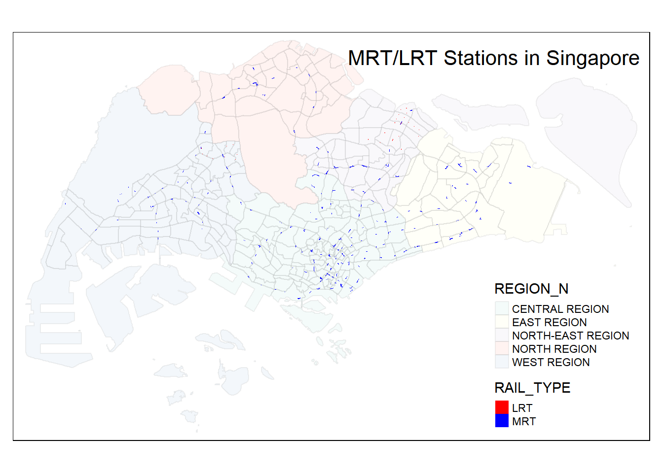
glimpse(geo_mrt_lrt_stn)Rows: 257
Columns: 7
$ Name <chr> "kml_1", "kml_2", "kml_3", "kml_4", "kml_5", "kml_6", "kml_…
$ GRND_LEVEL <chr> "ABOVEGROUND", "ABOVEGROUND", "UNDERGROUND", "ABOVEGROUND",…
$ RAIL_TYPE <chr> "LRT", "LRT", "MRT", "LRT", "LRT", "LRT", "LRT", "MRT", "LR…
$ NAME <chr> "PUNGGOL CENTRAL", "KANGKAR", "SENGKANG", "PUNGGOL POINT", …
$ INC_CRC <chr> "5ED154CD47409638", "B4ACD980B1469EC8", "632967D234F4FBC1",…
$ FMEL_UPD_D <chr> "20191209180316", "20191209180316", "20191209180316", "2019…
$ geometry <MULTIPOLYGON [m]> MULTIPOLYGON (((35733.24 43..., MULTIPOLYGON (…Filter and view data
geo_stn_na <- filter(geo_mrt_lrt_stn,NAME == "")
geo_stn_naSimple feature collection with 9 features and 6 fields
Geometry type: MULTIPOLYGON
Dimension: XY
Bounding box: xmin: 26284.4 ymin: 26002.6 xmax: 31443.34 ymax: 32930.38
Projected CRS: SVY21 / Singapore TM
Name GRND_LEVEL RAIL_TYPE NAME INC_CRC FMEL_UPD_D
1 kml_74 ABOVEGROUND LRT 6E7738D952D979E6 20191209180316
2 kml_75 ABOVEGROUND LRT 063BB9671365F6AE 20191209180316
3 kml_77 UNDERGROUND MRT 77802D2E751C9B73 20191209180316
4 kml_80 UNDERGROUND MRT A090AC90C1A289F3 20191209180316
5 kml_92 UNDERGROUND MRT 16771CD5289886F0 20191209180316
6 kml_97 UNDERGROUND MRT D49FFB88DCDF2480 20191209180316
7 kml_107 ABOVEGROUND LRT 1AC0878EDEF194AC 20191209180316
8 kml_150 UNDERGROUND MRT 629E735F6C7BBF76 20191209180316
9 kml_203 UNDERGROUND MRT F129512398A35F02 20191209180316
geometry
1 MULTIPOLYGON (((26459.27 26...
2 MULTIPOLYGON (((26284.4 260...
3 MULTIPOLYGON (((30163.74 29...
4 MULTIPOLYGON (((29285.32 29...
5 MULTIPOLYGON (((28521.81 32...
6 MULTIPOLYGON (((29188.18 29...
7 MULTIPOLYGON (((26636.92 26...
8 MULTIPOLYGON (((31385.21 28...
9 MULTIPOLYGON (((26920.72 31...View on a map
tmap_mode("view") +
tm_shape(mpsz) +
tm_polygons("REGION_N", alpha = 0.1, border.alpha = 0.1) +
tm_shape(geo_stn_na) +
tm_fill("Name", palette =c("red", "blue"), popup.vars=c("NAME" = "NAME"))From the map and data above, we can see 9 stations has its names missing as shown below:
| Name (KML Name) | NAME (Station Name) |
|---|---|
| kml_74 | Imbiah (Sentosa Express) |
| kml_75 | Beach (Sentosa Express) |
| kml_77 | Downtown (DTL) |
| kml_80 | Chinatown (DTL) |
| kml_92 | Newton (DTL) |
| kml_97 | Maxwell (TEL) |
| kml_107 | Waterfront (Sentosa Express) |
| kml_150 | Marina East (TEL) |
| kml_203 | Orchard Boulevard (TEL) |
We don’t want the Sentosa Express data as it serves more for leisure purpose. We will drop it from the dataframe later.
Fixing Data
geo_mrt_lrt_stn[geo_mrt_lrt_stn$Name == "kml_74", "NAME"] <- "IMBIAH"
geo_mrt_lrt_stn[geo_mrt_lrt_stn$Name == "kml_75", "NAME"] <- "BEACH"
geo_mrt_lrt_stn[geo_mrt_lrt_stn$Name == "kml_77", "NAME"] <- "DOWNTOWN"
geo_mrt_lrt_stn[geo_mrt_lrt_stn$Name == "kml_80", "NAME"] <- "CHINATOWN"
geo_mrt_lrt_stn[geo_mrt_lrt_stn$Name == "kml_92", "NAME"] <- "NEWTON"
geo_mrt_lrt_stn[geo_mrt_lrt_stn$Name == "kml_97", "NAME"] <- "MAXWELL"
geo_mrt_lrt_stn[geo_mrt_lrt_stn$Name == "kml_107", "NAME"] <- "WATERFRONT"
geo_mrt_lrt_stn[geo_mrt_lrt_stn$Name == "kml_150", "NAME"] <- "MARINA SOUTH"
geo_mrt_lrt_stn[geo_mrt_lrt_stn$Name == "kml_203", "NAME"] <- "ORCHARD BOULEVARD"There are a few steps to obtaining the data in the format we want.
We want the data in three dataframes:
- Existing MRT stations - North South Line, East West Line, Changi Airport Line, North East Line, Circle Line, Downtown Line, Thomson East Coast Line 1, 2 and 3
- Existing LRT stations - Bukit Panjang LRT, Sengkang LRT, Punggol LRT
- Future MRT stations - Thomson East Coast Line 4, 5, Jurong Region Line, Cross Island Line 1, Punggol Extension (we need to manually insert the stations)
The reason why Cross Island Line 2 was not included is that it is only announced on 20 Sep 2022 which is outside of our model data range. Hence, those stations would not have affected the housing prices in any way. We also want to exclude stations that do not have a definite opening date (Bukit Brown, Marina South and Mount Pleasant).
There are also a few other hurdles we need to go through:
- Interchange MRT stations have multiple polygons and records, we need to merge them
- For our analysis, we want to convert the polygons to points to be able to perform our analysis.
3.3.4 Extraction of Data into Different DataFrames
FUTURE_MRT = c("CHOA CHU KANG WEST", "TENGAH", "TENGAH PLANTATION", "TENGAH PARK", "BUKIT BATOK WEST", "TOH GUAN", "JURONG TOWN HALL", "PANDAN RESERVOIR", "HONG KAH", "CORPORATION", "JURONG WEST", "BAHAR JUNCTION", "GEK POH", "TAWAS", "NANYANG GATEWAY", "NANYANG CRESCENT", "PENG KANG HILL", "ENTERPRISE", "TUKANG", "JURONG HILL", "JURONG PIER", "FOUNDERS' MEMORIAL", "TANJONG RHU", "KATONG PARK", "TANJONG KATONG", "MARINE PARADE", "MARINE TERRACE", "SIGLAP", "BAYSHORE", "BEDOK SOUTH", "SUNGEI BEDOK", "XILIN", "AVIATION PARK", "LOYANG", "PASIR RIS EAST", "TAMPINES NORTH", "DEFU", "SERANGOON NORTH", "TAVISTOCK", "TECK GHEE", "HUME", "KEPPEL", "CANTONMENT", "PRINCE EDWARD ROAD", "PUNGGOL COAST")
EXCLUDE = c("MARINA SOUTH", "BUKIT BROWN", "MOUNT PLEASANT", "WATERFRONT", "BEACH", "IMBIAH")
geo_mrt_future <- geo_mrt_lrt_stn %>%
filter(NAME %in% FUTURE_MRT)
glimpse(geo_mrt_future)Rows: 45
Columns: 7
$ Name <chr> "kml_112", "kml_113", "kml_114", "kml_115", "kml_117", "kml…
$ GRND_LEVEL <chr> "UNDERGROUND", "UNDERGROUND", "UNDERGROUND", "UNDERGROUND",…
$ RAIL_TYPE <chr> "MRT", "MRT", "MRT", "MRT", "MRT", "MRT", "MRT", "MRT", "MR…
$ NAME <chr> "KEPPEL", "PRINCE EDWARD ROAD", "MARINE TERRACE", "TANJONG …
$ INC_CRC <chr> "EB7F6899585EF37F", "39C6C15CF1F42E35", "82E332FCCD9A7844",…
$ FMEL_UPD_D <chr> "20191209180316", "20191209180316", "20191209180316", "2019…
$ geometry <MULTIPOLYGON [m]> MULTIPOLYGON (((27779.18 28..., MULTIPOLYGON (…Looks correct! We have 44 unique future MRT stations that are new (excludes new interchanges with existing lines), 1 unique station is Sungei Bedok which is an interchange on TEL and DTL, hence, 44 records.
geo_lrt <- geo_mrt_lrt_stn %>%
filter(RAIL_TYPE == "LRT") %>% filter(!NAME %in% EXCLUDE)
glimpse(geo_lrt)Rows: 42
Columns: 7
$ Name <chr> "kml_1", "kml_2", "kml_4", "kml_5", "kml_6", "kml_7", "kml_…
$ GRND_LEVEL <chr> "ABOVEGROUND", "ABOVEGROUND", "ABOVEGROUND", "ABOVEGROUND",…
$ RAIL_TYPE <chr> "LRT", "LRT", "LRT", "LRT", "LRT", "LRT", "LRT", "LRT", "LR…
$ NAME <chr> "PUNGGOL CENTRAL", "KANGKAR", "PUNGGOL POINT", "TONGKANG", …
$ INC_CRC <chr> "5ED154CD47409638", "B4ACD980B1469EC8", "933DB538DAED1131",…
$ FMEL_UPD_D <chr> "20191209180316", "20191209180316", "20191209180316", "2019…
$ geometry <MULTIPOLYGON [m]> MULTIPOLYGON (((35733.24 43..., MULTIPOLYGON (…Looks correct! We have 42 LRT stations in Singapore.
geo_mrt_existing <- geo_mrt_lrt_stn %>%
filter(RAIL_TYPE == "MRT") %>% filter(!NAME %in% EXCLUDE) %>% filter(!NAME %in% FUTURE_MRT)
geo_mrt_existingSimple feature collection with 164 features and 6 fields
Geometry type: MULTIPOLYGON
Dimension: XY
Bounding box: xmin: 6071.311 ymin: 27478.44 xmax: 45377.5 ymax: 47909.19
Projected CRS: SVY21 / Singapore TM
First 10 features:
Name GRND_LEVEL RAIL_TYPE NAME INC_CRC
1 kml_3 UNDERGROUND MRT SENGKANG 632967D234F4FBC1
2 kml_8 UNDERGROUND MRT SERANGOON INTERCHANGE 10AD56727C54F2E3
3 kml_10 UNDERGROUND MRT SERANGOON INTERCHANGE E7D5531A772135B5
4 kml_11 UNDERGROUND MRT HOUGANG INTERCHANGE 032485860BA27411
5 kml_20 ABOVEGROUND MRT ANG MO KIO INTERCHANGE D64E567C239205F5
6 kml_21 UNDERGROUND MRT BUANGKOK FD00A32769DEBB52
7 kml_25 UNDERGROUND MRT PUNGGOL 95F1A1BF2CBD6BAB
8 kml_32 UNDERGROUND MRT LORONG CHUAN 5FCC9E048B7E6A46
9 kml_33 UNDERGROUND MRT KOVAN 775AEAABC9BE428A
10 kml_34 UNDERGROUND MRT TAI SENG 0D7A0B79F3C6ED17
FMEL_UPD_D geometry
1 20191209180316 MULTIPOLYGON (((34864.22 41...
2 20191209180316 MULTIPOLYGON (((32441.88 36...
3 20191209180316 MULTIPOLYGON (((32244.31 36...
4 20191209180316 MULTIPOLYGON (((34598.99 39...
5 20191209180316 MULTIPOLYGON (((29843.49 39...
6 20191209180316 MULTIPOLYGON (((34646.22 40...
7 20191209180316 MULTIPOLYGON (((35594.52 42...
8 20191209180316 MULTIPOLYGON (((31301.07 37...
9 20191209180316 MULTIPOLYGON (((33691.69 37...
10 20191209180316 MULTIPOLYGON (((34040.35 35...By looking through the dataframe, the data looks correct!
3.3.4.1 Merging Polygons for Data Frame
For geo_mrt which contains data of existing MRT stations, there are interchange stations which has seperate polygons. For example, Dhoby Ghaut MRT station is an interchange between 3 lines and hence has 3 polygons and records as seen below:
filter(geo_mrt_existing, NAME == "DHOBY GHAUT INTERCHANGE")Simple feature collection with 3 features and 6 fields
Geometry type: MULTIPOLYGON
Dimension: XY
Bounding box: xmin: 29264.89 ymin: 31193.36 xmax: 29514.18 ymax: 31463.67
Projected CRS: SVY21 / Singapore TM
Name GRND_LEVEL RAIL_TYPE NAME INC_CRC
1 kml_156 UNDERGROUND MRT DHOBY GHAUT INTERCHANGE A6CB94C5971F5F03
2 kml_157 UNDERGROUND MRT DHOBY GHAUT INTERCHANGE 17D85BD34169ABF7
3 kml_158 UNDERGROUND MRT DHOBY GHAUT INTERCHANGE 72739458BF8AB3E7
FMEL_UPD_D geometry
1 20191209180316 MULTIPOLYGON (((29385.16 31...
2 20191209180316 MULTIPOLYGON (((29293.51 31...
3 20191209180316 MULTIPOLYGON (((29385.16 31...We want to merge the records to obtain a single spatial point for each MRT station. Below, we will identify the interchange stations and merge their records and polgons manually.
Function to merge 2 and 3 rows respectively
merge_2 <- function(df, kml_1, kml_2){
operation <- st_union(filter(df, Name == kml_1), filter(df, Name == kml_2))
operation <- select(operation, "geometry")
df[df$Name == kml_1, "geometry"] <- operation
df <- subset(df, Name != kml_2)
return(df)
}
merge_3 <- function(df, kml_1, kml_2, kml_3){
operation <- st_union(filter(df, Name == kml_1), filter(df, Name == kml_2))
operation <- select(operation, c(0:6, "geometry"))
operation <- st_union(operation, filter(df, Name == kml_3))
operation <- select(operation, "geometry")
df[df$Name == kml_1, "geometry"] <- operation
df <- subset(df, Name != kml_2)
df <- subset(df, Name != kml_3)
return(df)
}The polygons are merged for the stations as indicated in the code block
# ANG MO KIO
geo_mrt_existing <- merge_2(geo_mrt_existing, "kml_20", "kml_236")
# BISHAN
geo_mrt_existing <- merge_2(geo_mrt_existing, "kml_43", "kml_247")
# BOON LAY
geo_mrt_existing <- merge_2(geo_mrt_existing, "kml_180", "kml_205")
# BOTANIC GARDENS
geo_mrt_existing <- merge_2(geo_mrt_existing, "kml_210", "kml_211")
# BONUA VISTA
geo_mrt_existing <- merge_2(geo_mrt_existing, "kml_227", "kml_228")
# CALDECOTT
geo_mrt_existing <- merge_2(geo_mrt_existing, "kml_231", "kml_232")
# CHINATOWN
geo_mrt_existing <- merge_2(geo_mrt_existing, "kml_80", "kml_165")
# CHOA CHU KANG
geo_mrt_existing <- merge_2(geo_mrt_existing, "kml_118", "kml_187")
# DHOBY GHAUT
geo_mrt_existing <- merge_3(geo_mrt_existing, "kml_156", "kml_157", "kml_158")
# EXPO
geo_mrt_existing <- merge_2(geo_mrt_existing, "kml_108", "kml_174")
# HARBOURFRONT
geo_mrt_existing <- merge_2(geo_mrt_existing, "kml_58", "kml_59")
# HOUGANG
geo_mrt_existing <- merge_2(geo_mrt_existing, "kml_11", "kml_245")
# JURONG EAST
geo_mrt_existing <- merge_2(geo_mrt_existing, "kml_135", "kml_136")
# LITTLE INDIA
geo_mrt_existing <- merge_2(geo_mrt_existing, "kml_160", "kml_161")
# MACPHERSON
geo_mrt_existing <- merge_2(geo_mrt_existing, "kml_222", "kml_223")
# MARINA BAY
geo_mrt_existing <- merge_3(geo_mrt_existing, "kml_68", "kml_78", "kml_147")
geo_mrt_existing <- merge_2(geo_mrt_existing, "kml_68", "kml_148")
# NEWTON
geo_mrt_existing <- merge_2(geo_mrt_existing, "kml_72", "kml_92")
# ORCHARD
geo_mrt_existing <- merge_2(geo_mrt_existing, "kml_98", "kml_154")
# OUTRAM PARK
geo_mrt_existing <- merge_3(geo_mrt_existing, "kml_100", "kml_151", "kml_251")
# PASIR RIS
geo_mrt_existing <- merge_2(geo_mrt_existing, "kml_239", "kml_243")
# PAYA LEBAR
geo_mrt_existing <- merge_2(geo_mrt_existing, "kml_153", "kml_212")
# SERANGOON
geo_mrt_existing <- merge_2(geo_mrt_existing, "kml_8", "kml_10")
# STEVENS
geo_mrt_existing <- merge_2(geo_mrt_existing, "kml_105", "kml_209")
# TAMPINES
geo_mrt_existing <- merge_2(geo_mrt_existing, "kml_35", "kml_166")
# WOODLANDS
geo_mrt_existing <- merge_2(geo_mrt_existing, "kml_64", "kml_169")
# BUGIS
geo_mrt_existing <- merge_2(geo_mrt_existing, "kml_81", "kml_70")That’s right, we have 134 unique existing MRT stations
3.3.4.2 Converting Spatial Polygons to Spatial Points
geo_mrt_existing <- st_centroid(geo_mrt_existing)
geo_lrt <- st_centroid(geo_lrt)
geo_mrt_future <- st_centroid(geo_mrt_future)3.3.4.3 Insert Cross Island Line Punggol Future Stations
The Master Plan 2019 MRT/LRT Station data excludes the Cross Island Line Punggol Stations, so we have to add them. 2 New MRT stations (that are not an existing interchange station with existing lines needs to be added). These are: Riveriaand Elias
new_df <- data.frame(Name = "kml_998", GRND_LEVEL = "UNDERGROUND", RAIL_TYPE = "MRT", NAME = "ELIAS", INC_CRC = "", FMEL_UPD_D = "", lng = "103.984", lat = "1.384")
new_df_coords <- st_as_sf(new_df, coords = c("lng", "lat"), crs=4326)
new_df_coords <- new_df_coords %>% st_transform(3414)
geo_mrt_future <- rbind(new_df_coords, geo_mrt_future)
new_df <- data.frame(Name = "kml_999", GRND_LEVEL = "UNDERGROUND", RAIL_TYPE = "MRT", NAME = "RIVERIA", INC_CRC = "", FMEL_UPD_D = "", lng = "103.916772", lat = "1.394439")
new_df_coords <- st_as_sf(new_df, coords = c("lng", "lat"), crs=4326)
new_df_coords <- new_df_coords %>% st_transform(3414)
geo_mrt_future <- rbind(new_df_coords, geo_mrt_future)3.3.5 Verifying MRT/LRT Data
tmap_mode("plot") +
tm_shape(mpsz) +
tm_polygons("REGION_N", alpha = 0.05, border.alpha = 0.05) +
tm_shape(geo_mrt_existing) +
tm_dots("RAIL_TYPE", palette = "darkgreen", title = "Existing MRT", size = 0.02) +
tm_shape(geo_lrt) +
tm_dots("RAIL_TYPE", palette = "blue", title = "Existing LRT", size = 0.02) +
tm_shape(geo_mrt_future) +
tm_dots("RAIL_TYPE", palette = "red", title = "Future MRT", size = 0.02) +
tm_layout(legend.position = c("right", "bottom"),
title= 'MRT/LRT Stations in Singapore',
title.position = c('right', 'top'))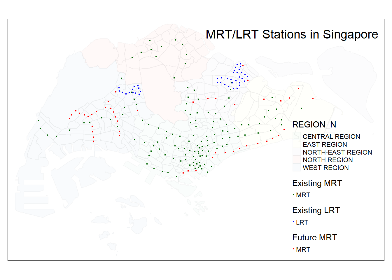
Everything looks to be plotted correctly.
3.3.6 Transforming Railway Line
tmap_mode("plot") +
tm_shape(mpsz) +
tm_polygons("REGION_N", alpha = 0.05, border.alpha = 0.05) +
tm_shape(geo_railway_line) +
tm_lines(c("GRND_LEVEL", "RAIL_TYPE"), palette = c("red", "blue", "darkgreen")) +
tm_layout(legend.position = c("right", "bottom"),
title= 'Railway Line in Singapore',
title.position = c('right', 'top'))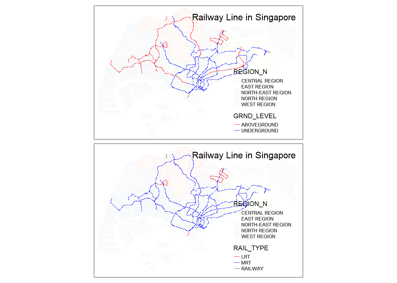
As we can see from our tmap plot above, the dataset contains:
GRND_LEVEL- Whether the track segment is above or undergroundRAIL_TYPE- Whether the track belongs toLRT,MRTorRAILWAY(KTM train)
Do note that since the data is extracted from URA Master Plan 2019 Rail Line, we will be able to see all current and future rail lines (Thomson East Coast Lines Stages 4, 5, Cross Island Line 1, Jurong Region Line).
For our analysis, we only want the above ground segments, seperated by RAIL_TYPE but excluding KTM data, as generally above ground segments affects residents the most. The reason why we seperate it by RAIL_TYPE is that LRT makes lesser noise than MRT and may not adversely impact housing prices as much as MRT. For MRTs, NUS researchers found that housing values were impacted by noise.
The rationale of including future aboveground lines like the Jurong Region Line in our analysis is that housing prices could be affected by the construction or announcement of future MRT lines which may cause housing prices to fall.
3.3.6.1 Splitting MRT/LRT Datasets
MRT
geo_rail_mrt_above <- geo_railway_line %>% filter(GRND_LEVEL == "ABOVEGROUND") %>% filter(RAIL_TYPE == "MRT")LRT
geo_rail_lrt_above <- geo_railway_line %>% filter(GRND_LEVEL == "ABOVEGROUND") %>% filter(RAIL_TYPE == "LRT")MRT
glimpse(geo_rail_mrt_above)Rows: 341
Columns: 6
$ Name <chr> "kml_1", "kml_4", "kml_5", "kml_6", "kml_7", "kml_24", "kml…
$ GRND_LEVEL <chr> "ABOVEGROUND", "ABOVEGROUND", "ABOVEGROUND", "ABOVEGROUND",…
$ RAIL_TYPE <chr> "MRT", "MRT", "MRT", "MRT", "MRT", "MRT", "MRT", "MRT", "MR…
$ INC_CRC <chr> "19247B0E0E15AF87", "4E3C7F23EFA39E37", "F49903A9C3D88B3E",…
$ FMEL_UPD_D <chr> "20191209172332", "20191209172332", "20191209172332", "2019…
$ geometry <MULTILINESTRING [m]> MULTILINESTRING ((20846.61 ..., MULTILINEST…LRT
glimpse(geo_rail_lrt_above)Rows: 116
Columns: 6
$ Name <chr> "kml_60", "kml_61", "kml_62", "kml_63", "kml_73", "kml_319"…
$ GRND_LEVEL <chr> "ABOVEGROUND", "ABOVEGROUND", "ABOVEGROUND", "ABOVEGROUND",…
$ RAIL_TYPE <chr> "LRT", "LRT", "LRT", "LRT", "LRT", "LRT", "LRT", "LRT", "LR…
$ INC_CRC <chr> "91095B49D361DDB8", "C00FE7321D9283D7", "828BF093EA1BA1A8",…
$ FMEL_UPD_D <chr> "20191209172332", "20191209172332", "20191209172332", "2019…
$ geometry <MULTILINESTRING [m]> MULTILINESTRING ((26936.7 2..., MULTILINEST…3.3.6.2 Verifying MRT/LRT Aboveground Railway Line
tmap_mode("plot") +
tm_shape(mpsz) +
tm_polygons("REGION_N", alpha = 0.05, border.alpha = 0.05) +
tm_shape(geo_rail_mrt_above) +
tm_lines("RAIL_TYPE", palette = "red") +
tm_shape(geo_rail_lrt_above) +
tm_lines("RAIL_TYPE", palette = "blue") +
tm_layout(legend.position = c("right", "bottom"),
title= 'MRT/LRT Track Line in Singapore',
title.position = c('right', 'top'))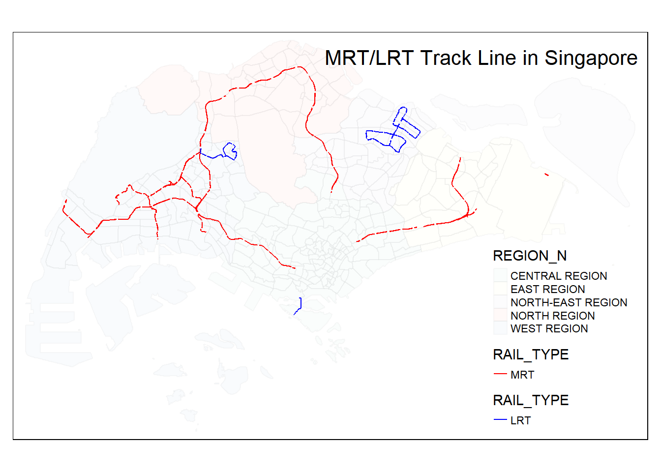
3.3.7 Transform Parks Dataset
Let us view our parks dataset
glimpse(geo_parks)Rows: 421
Columns: 3
$ Name <chr> "JANGGUS GARDEN", "JLN LIMAU MANIS PG", "GARDEN VIEW PG", …
$ Description <chr> "<html xmlns:fo=\"http://www.w3.org/1999/XSL/Format\" xmln…
$ geometry <MULTIPOLYGON [m]> MULTIPOLYGON (((28392.92 48..., MULTIPOLYGON …tmap_mode("plot") +
tm_shape(mpsz) +
tm_polygons("REGION_N", alpha = 0.05, border.alpha = 0.05) +
tm_shape(geo_parks) +
tm_fill("darkgreen") +
tm_layout(legend.position = c("right", "bottom"),
title= 'Parks in Singapore',
title.position = c('right', 'top'))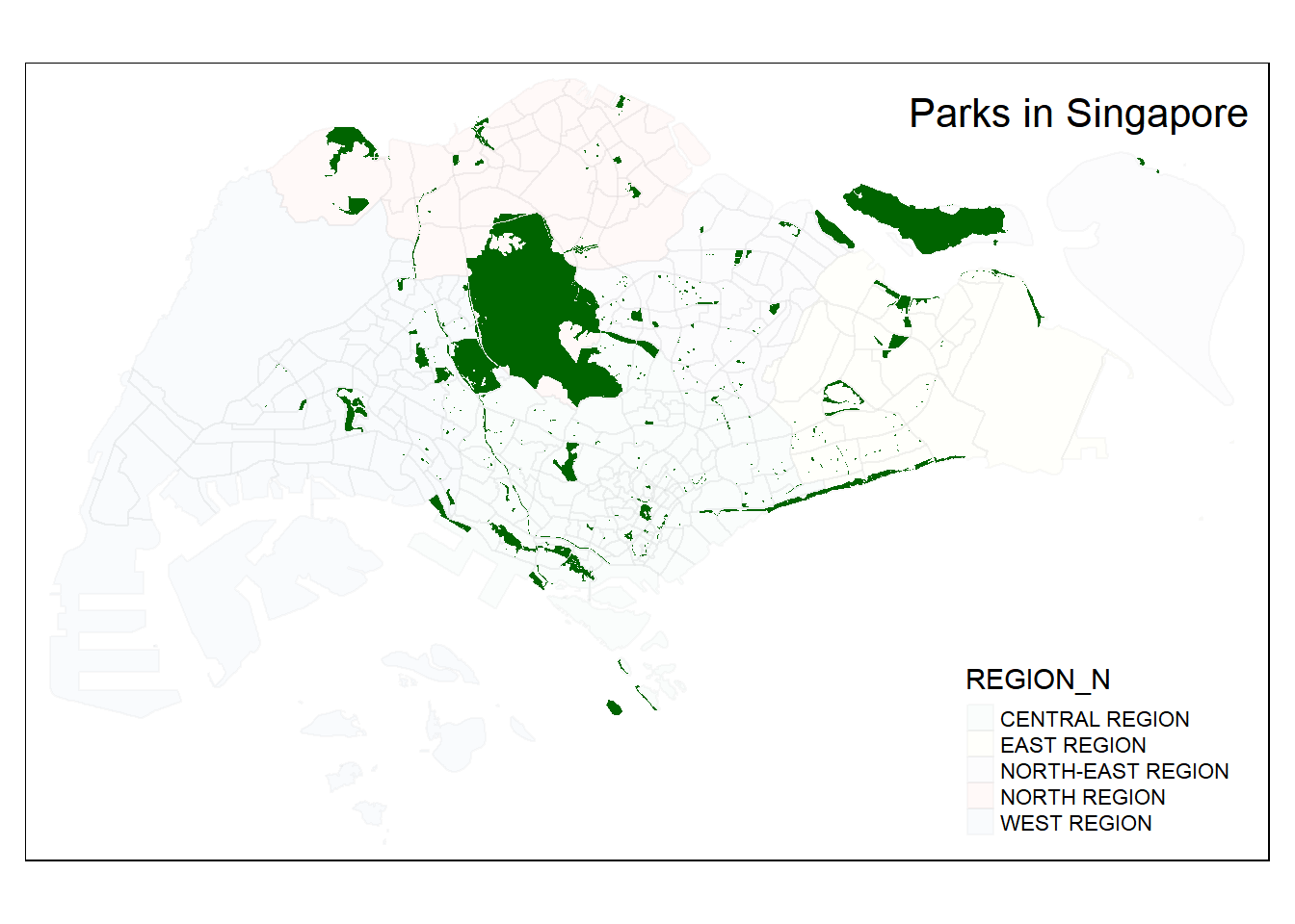
Firstly, as we recognise that parks comes in different shapes and sizes. Parks like Punggol Waterway Park are long by nature and spans the entire width of Punggol. Hence, using a Spatial Points by obtaining its centroid is not the most accurate as the entire length is a park. Hence, we opt to use the park polygon instead.
Our data is in the MULTIPOLYGON format. As we want to calculate the proximity from homes to the edges of parks, we need to convert it to LINESTRING. The code block uses st_cast() to help us cast the format from MULTIPOLYGON to LINESTRING
geo_parks <- geo_parks %>% st_cast("MULTILINESTRING") %>% st_cast("LINESTRING")Now, let us check and plot the map of the parks data.
glimpse(geo_parks)Rows: 687
Columns: 3
$ Name <chr> "JANGGUS GARDEN", "JLN LIMAU MANIS PG", "GARDEN VIEW PG", …
$ Description <chr> "<html xmlns:fo=\"http://www.w3.org/1999/XSL/Format\" xmln…
$ geometry <LINESTRING [m]> LINESTRING (28392.92 48794...., LINESTRING (408…tmap_mode("plot") +
tm_shape(mpsz) +
tm_polygons("REGION_N", alpha = 0.05, border.alpha = 0.05) +
tm_shape(geo_parks) +
tm_lines("darkgreen") +
tm_layout(legend.position = c("right", "bottom"),
title= 'Parks in Singapore',
title.position = c('right', 'top'))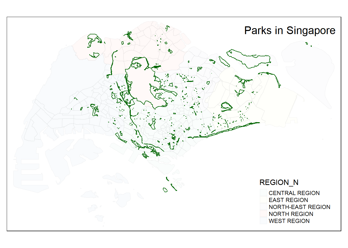
Great! We have successfully converted the data to LINESTRING!
3.3.8 Prepare Good Primary Schools Dataset
schlah.com provides a good breakdown of factors that contributes to a school’s ranking, based on the following extracted from their website:
Gifted Education Programme (GEP): 20%
Popularity in Primary 1 (P1) Registration: 20%
Special Assistance Plan (SAP): 15%
Singapore Youth Festival Arts Presentation: 15%
Singapore National School Games: 15%
Singapore Uniformed Groups Unit Recognition: 15%
In our analysis, we want to see if good schools can contribute to increased housing prices in Singapore. For our analysis, we will take that the top 10% (16) of primary schools in Singapore are ‘good schools’
The code chunk below will extract the top 16 good primary schools for our analysis.
TOP_10PCT_SCHS = c("NANYANG PRIMARY SCHOOL",
"TAO NAN SCHOOL",
"CATHOLIC HIGH SCHOOL",
"NAN HUA PRIMARY SCHOOL",
"ST. HILDA'S PRIMARY SCHOOL",
"HENRY PARK PRIMARY SCHOOL",
"ANGLO-CHINESE SCHOOL (PRIMARY)",
"RAFFLES GIRLS' PRIMARY SCHOOL",
"PEI HWA PRESBYTERIAN PRIMARY SCHOOL",
"CHIJ ST. NICHOLAS GIRLS' SCHOOL",
"ROSYTH SCHOOL",
"KONG HWA SCHOOL",
"POI CHING SCHOOL",
"HOLY INNOCENTS' PRIMARY SCHOOL",
"AI TONG SCHOOL",
"RED SWASTIKA SCHOOL")
geo_top_schools = geo_schools %>% filter(SCHOOLNAME %in% TOP_10PCT_SCHS)
glimpse(geo_top_schools)Rows: 16
Columns: 14
$ SCHOOLNAME <chr> "AI TONG SCHOOL", "ANGLO-CHINESE SCHOOL (PRIMARY)", "C…
$ SCH_HSE_BLK_NUM <chr> "100", "50", "9", "501", "1", "5", "350", "30", "52", …
$ HSE_BLK_NUM <chr> "100", "50", "9", "501", "1", "5", "350", "30", "52", …
$ SCH_POSTAL_CODE <chr> "579646", "309918", "579767", "569405", "278790", "536…
$ POSTAL_CODE <chr> "579646", "309918", "579767", "569405", "278790", "536…
$ SCH_ROAD_NAME <chr> "BRIGHT HILL DRIVE", "BARKER ROAD", "BISHAN STREET 22"…
$ ROAD_NAME <chr> "BRIGHT HILL DRIVE", "BARKER ROAD", "BISHAN STREET 22"…
$ HYPERLINK <chr> "", "", "", "", "", "", "", "", "", "", "", "", "", ""…
$ MOREINFO <chr> "https://www.moe.gov.sg/schoolfinder", "https://www.mo…
$ LATITUDE <chr> "1.3606564354832", "1.3187690519982", "1.3548563617849…
$ LONGITUDE <chr> "103.83293164489", "103.83570184821", "103.84376151132…
$ GEOMETRY <chr> "{{hG_vvxRTAhDEJCFIdAeDFMHKJKJGBCIS_EoAADABEHEHINGL?@C…
$ SCH_TEXT <chr> "Ai Tong Sch", "Anglo-Chinese Sch (Pri)", "Catholic Hi…
$ geometry <POINT [m]> POINT (27956.94 38079.99), POINT (28265.23 33448…There we have it, we have successfully extracted the top 10% of primary schools in Singapore (16 schools).
3.3.9 Prepare CBD Outline
From Wikipedia, we know that Singapore’s CBD is also called DOWNTOWN CORE. To be accurate in our analysis, we will calculate the proximity to CBD based on the following rules:
if outside CBD boundary, we will calcualte the distance to the
LINESTRING.if within CBD, distance will be 0
The codeblock below achieves a few things:
- Filter to get the subzones of
DOWNTOWN COREplanning area - Combine the polygons to obtain the outline of
DOWNTOWN CORE(CBD) - Convert the geometry from
POLYGONtoLINESTRINGformat
cbd_sf <- mpsz %>% filter(mpsz$PLN_AREA_N == "DOWNTOWN CORE")
cbd_geom <- st_union(cbd_sf)
cbd_geom <- st_cast(cbd_geom, "LINESTRING")4 Data Wrangling: Aspatial Data
We have three datasets that are Aspatial Data which only contains addresses of the locations. However, we cannot perform analysis without the coordinates of the datasets without its coordinates, hence, we need to geocode the data to retrieve its coordinates using onemap.
These are the datasets that require further processing:
CHAS Clinics
HDB HIP MUP
HDB Resale Flat Pricing
Shopping Malls
4.1 Importing Aspatial Data
In the various tabs below, we will import each individual dataset from its respective folders, with a brief explanation of the use cases of each dataset.
CHAS_raw = read_xlsx("Take-Home_Ex03/aspatial/CHAS.xlsx")
glimpse(CHAS_raw)Rows: 1,910
Columns: 7
$ Name <chr> "1 Aljunied Medical", "1 BISHAN MEDICAL", "1 ME…
$ Address <chr> "Singapore 367874", "283, Bishan Street, #01- 1…
$ Postal <chr> "367874", "570283", "560410", "560704", "600135…
$ Telephone <chr> NA, "64561600", "62517030", "96311728", "977017…
$ Type <chr> "Medical", "Medical, Cervical\r\nCancer Screen"…
$ Website <chr> NA, NA, NA, NA, NA, NA, NA, NA, NA, NA, NA, NA,…
$ `Pap Test\r\nServices` <chr> "No", "Yes", "No", "No", "No", "No", "No", "No"…hdb_hip_mup_raw = read_xlsx("Take-Home_Ex03/aspatial/HDB_HIP-MUP-20230312.xlsx")
glimpse(hdb_hip_mup_raw)Rows: 2,769
Columns: 4
$ BLK <chr> "218", "219", "220", "221", "222", "223", "225", "226", "226B",…
$ STREET <chr> "ANG MO KIO AVE 1", "ANG MO KIO AVE 1", "ANG MO KIO AVE 1", "AN…
$ TYPE <chr> "HIP", "HIP", "HIP", "HIP", "HIP", "HIP", "HIP", "HIP", "HIP", …
$ TOWN <chr> "ANG MO KIO", "ANG MO KIO", "ANG MO KIO", "ANG MO KIO", "ANG MO…hdb_resale_raw = read_csv("Take-Home_Ex03/aspatial/resale-flat-prices-based-on-registration-date-from-jan-2017-onwards.csv")
glimpse(hdb_resale_raw)Rows: 148,373
Columns: 11
$ month <chr> "2017-01", "2017-01", "2017-01", "2017-01", "2017-…
$ town <chr> "ANG MO KIO", "ANG MO KIO", "ANG MO KIO", "ANG MO …
$ flat_type <chr> "2 ROOM", "3 ROOM", "3 ROOM", "3 ROOM", "3 ROOM", …
$ block <chr> "406", "108", "602", "465", "601", "150", "447", "…
$ street_name <chr> "ANG MO KIO AVE 10", "ANG MO KIO AVE 4", "ANG MO K…
$ storey_range <chr> "10 TO 12", "01 TO 03", "01 TO 03", "04 TO 06", "0…
$ floor_area_sqm <dbl> 44, 67, 67, 68, 67, 68, 68, 67, 68, 67, 68, 67, 67…
$ flat_model <chr> "Improved", "New Generation", "New Generation", "N…
$ lease_commence_date <dbl> 1979, 1978, 1980, 1980, 1980, 1981, 1979, 1976, 19…
$ remaining_lease <chr> "61 years 04 months", "60 years 07 months", "62 ye…
$ resale_price <dbl> 232000, 250000, 262000, 265000, 265000, 275000, 28…shopping_malls_raw = read_xlsx("Take-Home_Ex03/aspatial/malls-20230320.xlsx")4.2 Filtering HDB Resale Flat Data
We will now filter the HDB Resale to focus on the target months, Jan 2021 to Feb 2023, and 5 Room HDBs to construct the predictive model. We will use:
filter() to filter out the desired room type and months
unique() to check if the desired room type and months has been filtered correctly
glimpse() to check the data structure of the filtered dataset
hdb_resale <- filter(hdb_resale_raw, flat_type == "5 ROOM") %>%
filter(month >= "2021-01" & month <= "2023-02")glimpse(hdb_resale)Rows: 15,516
Columns: 11
$ month <chr> "2021-01", "2021-01", "2021-01", "2021-01", "2021-…
$ town <chr> "ANG MO KIO", "ANG MO KIO", "ANG MO KIO", "ANG MO …
$ flat_type <chr> "5 ROOM", "5 ROOM", "5 ROOM", "5 ROOM", "5 ROOM", …
$ block <chr> "551", "305", "520", "253", "423", "617", "315A", …
$ street_name <chr> "ANG MO KIO AVE 10", "ANG MO KIO AVE 1", "ANG MO K…
$ storey_range <chr> "01 TO 03", "13 TO 15", "16 TO 18", "07 TO 09", "0…
$ floor_area_sqm <dbl> 118, 123, 118, 128, 133, 133, 110, 110, 110, 112, …
$ flat_model <chr> "Improved", "Standard", "Improved", "Improved", "I…
$ lease_commence_date <dbl> 1981, 1977, 1980, 1996, 1993, 1996, 2006, 2002, 20…
$ remaining_lease <chr> "59 years 01 month", "55 years 07 months", "58 yea…
$ resale_price <dbl> 483000, 590000, 629000, 670000, 680000, 760000, 76…unique(hdb_resale$month) [1] "2021-01" "2021-02" "2021-03" "2021-04" "2021-05" "2021-06" "2021-07"
[8] "2021-08" "2021-09" "2021-10" "2021-11" "2021-12" "2022-01" "2022-02"
[15] "2022-03" "2022-04" "2022-05" "2022-06" "2022-07" "2022-08" "2022-09"
[22] "2022-10" "2022-11" "2022-12" "2023-01" "2023-02"unique(hdb_resale$flat_type)[1] "5 ROOM"From the code and results in the respective tabs (Glimpse Variables and Unique Month and Flat Type), we can see that:
There are 21,500 transactions between Jan 2020 to Feb 2023.
The
monthandflat_typehas been extracted correctly.
4.3 Transforming Aspatial Data - Create New Columns with Values
Next, we transform the Aspatial Datasets into more meaningful values:
- CHAS Clinics - There is nothing to transform, since as noted earlier, there is already a
postalcolumn provided - HDB HIP MUP - We need to obtain the address for geocoding (obtaining the SVY21
XandYcoordinates) by combining theBLKandSTREETfields - HDB Resale Flat Pricing - We need to obtain the address for geocoding (obtaining the SVY21
XandYcoordinates) by combining theblockandstreet_namefields, and also convert the remaining lease from the form ofYY years MM monthsto a more machine-readable format (ie.MMmonths) - Shopping Malls - Nothing to transform, we can use the
Mall_Nameas the search term to obtain the geocode (SVYXandYcoordinates)
The code chunks will assist with the transformation using mutate() further explained below:
We mutate() the hdb_hip_mup_raw dataset by pasting the BLK and STREET columns together into the address column to a new sf dataframe called hdb_hip_mup_trans
hdb_hip_mup_trans <- hdb_hip_mup_raw %>%
mutate(hdb_hip_mup_raw, address = paste(BLK, STREET))We mutate() the hdb_resale dataset by pasting the block and street_name columns together into the address column to a new variable called hdb_hip_mup_trans. We also used mutate() to modify the existing remaining_lease data to the form of MM.
The first section of the code as.integer(str_sub(remaining_lease, 0, 2)) * 12 extracts the year numbers as YY and converts it into string and then multiplying it by 12 to convert it to number of months.
The next part of the code checks if there is any numerical MM (month) present, if there is no month present, the value will be NA and 0 will be assigned in place of NA. Else, if present, we take the MM.
The integer month is summed with the year in months to form this column remaining_lease_mths in the new sf dataframe hdb_resale_trans
hdb_resale_trans <- hdb_resale %>%
mutate(hdb_resale, address = paste(block, street_name)) %>%
mutate(hdb_resale, remaining_lease_mths = (as.integer(str_sub(remaining_lease, 0, 2)) * 12 + ifelse(is.na(as.integer(str_sub(remaining_lease, 9, 11))), 0, as.integer(str_sub(remaining_lease, 9, 11)))))Next, we also need to obtain the age of the HDBs. In Singapore, HDB leases are 99 years. We can take 99 - remaining_lease_mths to obtain age_of_unit_mths
hdb_resale_trans <- hdb_resale_trans %>% mutate(age_of_unit_mths = (99*12) - remaining_lease_mths)Next, let us left join the HDB HIP MUP data into HDB Resale Transactions so that we know which HDB units have already completed their upgrading.
hdb_resale_trans <- left_join(hdb_resale_trans, hdb_hip_mup_trans)
glimpse(hdb_resale_trans)Rows: 15,549
Columns: 18
$ month <chr> "2021-01", "2021-01", "2021-01", "2021-01", "2021…
$ town <chr> "ANG MO KIO", "ANG MO KIO", "ANG MO KIO", "ANG MO…
$ flat_type <chr> "5 ROOM", "5 ROOM", "5 ROOM", "5 ROOM", "5 ROOM",…
$ block <chr> "551", "305", "520", "253", "423", "617", "315A",…
$ street_name <chr> "ANG MO KIO AVE 10", "ANG MO KIO AVE 1", "ANG MO …
$ storey_range <chr> "01 TO 03", "13 TO 15", "16 TO 18", "07 TO 09", "…
$ floor_area_sqm <dbl> 118, 123, 118, 128, 133, 133, 110, 110, 110, 112,…
$ flat_model <chr> "Improved", "Standard", "Improved", "Improved", "…
$ lease_commence_date <dbl> 1981, 1977, 1980, 1996, 1993, 1996, 2006, 2002, 2…
$ remaining_lease <chr> "59 years 01 month", "55 years 07 months", "58 ye…
$ resale_price <dbl> 483000, 590000, 629000, 670000, 680000, 760000, 7…
$ address <chr> "551 ANG MO KIO AVE 10", "305 ANG MO KIO AVE 1", …
$ remaining_lease_mths <dbl> 709, 667, 704, 891, 855, 894, 1012, 971, 1012, 10…
$ age_of_unit_mths <dbl> 479, 521, 484, 297, 333, 294, 176, 217, 176, 113,…
$ BLK <chr> "551", "305", "520", NA, "423", NA, NA, NA, NA, N…
$ STREET <chr> "ANG MO KIO AVE 10", "ANG MO KIO AVE 1", "ANG MO …
$ TYPE <chr> "HIP", "MUP", "HIP", NA, "MUP", NA, NA, NA, NA, N…
$ TOWN <chr> "ANG MO KIO", "ANG MO KIO", "ANG MO KIO", NA, "AN…Then we’ll select only the unnecessary columns:
hdb_resale_trans <- hdb_resale_trans %>% select(c(1:14, 17))4.4 Retrieving SVY21 Coordinate of Addresses
This section will focus on retrieving relavant data such as coordinates of the address which we could use in further spatial analysis to obtain proximity to locational factors later.
We are interested in obtaining the SVY21 X and Y coordinates as they are in the Projected Coordinate System, which allows us to perform measure directly without any additional transformations.
4.4.1 Create a List Storing Unique Addresses/Postal Codes
Since some addresses/postal codes are duplicated, we store and check unique addresses to reduce the amount of GET requests sent to the OneMap API:
- Faster
- OneMap API has a rate limit of 250 API calls a minute
- It makes it easier for us to locate errors and correct it
Here, we will obtain a list of unique addresses/postal codes for each data set.
addr_lst.chas <- sort(unique(CHAS_raw$Postal))
glimpse(addr_lst.chas) chr [1:1128] "018935" "018972" "018981" "018982" "018984" "018987" ...addr_lst.resale <- sort(unique(hdb_resale_trans$address))
glimpse(addr_lst.resale) chr [1:4037] "1 CHAI CHEE RD" "1 DELTA AVE" "1 EVERTON PK" "1 MARINE TER" ...addr_lst.malls <- sort(unique(shopping_malls_raw$Mall_Name))
glimpse(addr_lst.malls) chr [1:166] "100 AM" "313@Somerset" "321 Clementi" "888 Plaza" ...4.4.2 Create Function to Retrieve Coordinates from OneMap.sg API
The following function uses OneMap.sg Search API to obtain coordinates (SVY21 X, Y) using part of an address or postal code.
This is how the function get_coordinates() below will work:
new_coordsdatafame is created to store all the new coordinate data and its original address that is input to the GET request API- for each
addrinaddr_lstwhereaddr_lstis the list passed into the function, we will query each record and append accordingly:If there is 1 or more records, we append the top record’s SVY21 X, Y coordinates and
addrto a temporary dataframe callednew_row,Else,
NAfor it’sXandYcolumns and theaddris stored innew_row.
- The GET Request has various parameters:
searchVal- the value to pass to OneMap Search to obtain the Geocode (in this case we are interested in SVY21 X, Y coordinates)returnGeom- return details about geometry (ie. SVY21 X, Y or Lat Lon),Yin this case as we want SVY21 X, Y coordinatesgetAddrDetails- get more details about the address,Nin this case as we don’t require further information.
- fromJSON() helps us convert the JSON format to a list format for manipulation
- the function rawToChar() was used as the received type for
reply$contentis RAW, which requires conversion before we can read the values
- the function rawToChar() was used as the received type for
- Lastly, we will combine the
new_rowdata into the mainnew_coordsdataframe using rbind() as they are both dataframes.
get_coordinates <- function(addr_lst){
# Create a data frame to store all retrieved coordinates
new_coords <- data.frame()
for (addr in addr_lst){
#print(i)
reply <- GET('https://developers.onemap.sg/commonapi/search?',
query = list(searchVal = addr,
returnGeom = 'Y',
getAddrDetails = 'N'))
output <- fromJSON(rawToChar(reply$content))
found <- output$found
res <- output$results
# Create a new data frame for each address
new_row <- data.frame()
# If single result, append
if (found >= 1){
res_1 <- head(res, n = 1)
x <- res_1$X
y <- res_1$Y
new_row <- data.frame(address = addr, x = x, y = y)
}
else {
new_row <- data.frame(address = addr, x = NA, y = NA)
}
# Add the row
new_coords <- rbind(new_coords, new_row)
}
return(new_coords)
}4.4.3 Call get_coordinates() Function to Obtain Coordinates
We use get_coordinates() function created earlier to obtain the coordinates of the address. glimpse() allows us to view and check if the data has been properly created.
RDS Scripts contains scripts to import/export the coordinates R objects to RDS file format (R Data Serialisation) prevent having to call the API each time on every render.
CHAS Clinics
coords_chas <- get_coordinates(addr_lst.chas)HDB Resale Flat Pricing
coords_resale <- get_coordinates(addr_lst.resale)Shopping Malls
coords_malls <- get_coordinates(addr_lst.malls)Writing RDS
write_rds(coords_chas, "Take-Home_Ex03/rds/coords_chas.rds")
write_rds(coords_resale, "Take-Home_Ex03/rds/coords_resale.rds")
write_rds(coords_malls, "Take-Home_Ex03/rds/coords_malls.rds")Reading RDS
coords_chas <- read_rds("Take-Home_Ex03/rds/coords_chas.rds")
coords_resale <- read_rds("Take-Home_Ex03/rds/coords_resale.rds")
coords_malls <- read_rds("Take-Home_Ex03/rds/coords_malls.rds")CHAS Clinics
glimpse(coords_chas)Rows: 1,128
Columns: 3
$ address <chr> "018935", "018972", "018981", "018982", "018984", "018987", "0…
$ x <chr> "30173.1125663621", "30856.1576845003", "30325.5481859585", "3…
$ y <chr> "28870.8731260244", "29629.71109147", "29166.1214467622", "290…HDB Resale Flat Pricing
glimpse(coords_resale)Rows: 4,283
Columns: 3
$ address <chr> "1 CHAI CHEE RD", "1 DELTA AVE", "1 EVERTON PK", "1 MARINE TER…
$ x <chr> "37949.0264732633", "27473.0907973954", "28899.2285061181", "3…
$ y <chr> "34465.7385691088", "30496.6361175738", "28663.7158067878", "3…Shopping Malls
glimpse(coords_malls)Rows: 166
Columns: 3
$ address <chr> "100 AM", "313@Somerset", "321 Clementi", "888 Plaza", "Admira…
$ x <chr> "29131.8164707171", "28561.1386390822", "20395.3064215332", "2…
$ y <chr> "28573.4721462838", "31485.0772309396", "32700.1500842664", "4…4.5 Data Verification for Coordinate Data
With the retrieved data, we need to inspect and verify the data received and correct any errors made along the way. We will do all the steps in parallel for each dataset, outlined in step format below:
- Merge coordinate data and original dataframe
- We do this as the CHAS Clinics coordinates are derived from Postal Code and it might be hard to figure out which place are we looking at by looking at just the postal code
- Check for
NAX/Y values and manually amend if required - Convert DataFrame into a sf Object
- Plot a tmap and check if points are plotted in the correct regions
At any step if there are issues, we will detail steps to fix or recover from it.
4.5.1 CHAS Clinics
Merge Coordinate Data and Original Dataframe
temp_chas <- left_join(CHAS_raw, coords_chas, by=c("Postal" = "address"))Check for
NAX/Y values and manually amend if requiredfilter(temp_chas, is.na(x) == TRUE)# A tibble: 8 × 9 Name Address Postal Telephone Type Website `Pap Test\r\nServices` x <chr> <chr> <chr> <chr> <chr> <chr> <chr> <chr> 1 "Atlantic… "189, … 188332 63387157 Dent… <NA> No <NA> 2 "DA CLINI… "140, … 610410 69541012 Medi… <NA> No <NA> 3 "Internat… "6, Ge… 69249 63720082 Dent… <NA> No <NA> 4 "Lifecare… "102, … 760102 67580453 Medi… <NA> No <NA> 5 "Lok Dent… "34, C… 089673 62250176 Dent… <NA> No <NA> 6 "People's… "1, Ro… 180001 62927629 Dent… <NA> No <NA> 7 "Raffles … "51, T… 529684 63112134 Medi… <NA> No <NA> 8 "Unity De… "50, M… 048940 65904400 Dent… <NA> No <NA> # ℹ 1 more variable: y <chr>Here, using filter() and is.na(), we find out which records do not have a valid location assigned to it. Now, let us manually check through the records and fix the issue.
CHAS Clinic Address Issue 189, Selegie Road, Selegie Centre, #01- 05, Singapore 188332 No longer exists based on Onemap and Google Map, we will remove it 140, Corporation Drive, #01- 03 Postal Code number 610140 according to OneMap, we will amend accordingly 6, Gemmill Lane Postal Code number 069249 according to OneMap, we will amend accordingly 102, Yishun Avenue 5, #01- 133, Singapore\r\n760102 No longer exists based on Onemap and Google Map, we will remove it 34, Craig Road, Chinatown Plaza, #01- 04,\r\nSingapore 089673 No longer exists based on Onemap and Google Map, we will remove it 1, Rochor Road, Rochor Centre, #03- 516,\r\nSingapore 180001 No longer exists based on Onemap and Google Map, we will remove it 51, TAMPINES AVENUE 4, OUR TAMPINES\r\nHUB, #B1- 04/05 Records are appended as 528523 on OneMap, we will amend accordingly 50, Market Street, Golden Shoe Car Park,\r\n#01- 30, Singapore 048940 No longer exists based on OneMap and Google Map, we will remove it Now, let us update:
4.5.1.1 Fixing Data
We remove the clinics that are non-existent using filter()
chas_updated <- filter(CHAS_raw, !Address %in% c("189, Selegie Road, Selegie Centre, #01- 05,\r\nSingapore 188332", "102, Yishun Avenue 5, #01- 133, Singapore\r\n760102", "34, Craig Road, Chinatown Plaza, #01- 04,\r\nSingapore 089673", "1, Rochor Road, Rochor Centre, #03- 516,\r\nSingapore 180001", "50, Market Street, Golden Shoe Car Park,\r\n#01- 30, Singapore 048940"))Next, we use mutate() and ifelse() condition to update the Postal Codes of the clinics at the relavant addresses.
chas_updated <- chas_updated %>% mutate(Postal = ifelse(Address == "140, Corporation Drive, #01- 03", "610140", Postal)) %>% mutate(Postal = ifelse(Address == "6, Gemmill Lane", "069249", Postal)) %>% mutate(Postal = ifelse(Address == "51, TAMPINES AVENUE 4, OUR TAMPINES\r\nHUB, #B1- 04/05", "528523", Postal))Lastly, we regenerate the list of unique Postal Codes to be geocoded.
addr_lst.chas_upd <- sort(unique(chas_updated$Postal)) glimpse(addr_lst.chas_upd)chr [1:1122] "018935" "018972" "018981" "018982" "018984" "018987" ...We get the SVY21 X,Y coordinates using our get_coordinates() function
coords_chas_upd <- get_coordinates(addr_lst.chas_upd)Saving the DataFrame as .rds for future use to prevent rerunning get_coordinates() GET API everytime a render is run
write_rds(coords_chas_upd, "Take-Home_Ex03/rds/coords_chas_upd.rds")Load the DataFrame from .rds
coords_chas_upd <- read_rds("Take-Home_Ex03/rds/coords_chas_upd.rds")We left join the
chas_updatedmain table and coordinates and filter thexcolumn for any null valuestemp_chas <- left_join(chas_updated, coords_chas_upd, by=c("Postal" = "address")) filter(temp_chas, is.na(x) == TRUE)# A tibble: 0 × 9 # ℹ 9 variables: Name <chr>, Address <chr>, Postal <chr>, Telephone <chr>, # Type <chr>, Website <chr>, Pap Test Services <chr>, x <chr>, y <chr>No null values found, we have completed this step!
Convert a DataFrame into a sf Object
We specify the SVY21 X and Y coordinates to be used as the coordinate geometry. The
crsspecified is3414which refers toSVY21.chas_sf <- st_as_sf(temp_chas, coords = c("x", "y"), crs = 3414)Plot a tmap and check if points are plotted in the correct regions
Now, we will plot an interactive tmap to check if our points are correct.
tmap_mode("view") tm_shape(chas_sf) + tm_dots("Type", popup.vars=c("Name"="Name", "Address"="Address", "Type" = "Type", "Telephone" = "Telephone"))From our analysis, the points looks to be correctly located.
4.5.2 HDB Resale Flat Pricing
Merge Coordinate Data and Original Dataframe
temp_hdb_resale_trans <- left_join(hdb_resale_trans, coords_resale, by=c("address" = "address"))Check for
NAX/Y values and manually amend if requiredfilter(temp_hdb_resale_trans, is.na(x) == TRUE)# A tibble: 0 × 17 # ℹ 17 variables: month <chr>, town <chr>, flat_type <chr>, block <chr>, # street_name <chr>, storey_range <chr>, floor_area_sqm <dbl>, # flat_model <chr>, lease_commence_date <dbl>, remaining_lease <chr>, # resale_price <dbl>, address <chr>, remaining_lease_mths <dbl>, # age_of_unit_mths <dbl>, TYPE <chr>, x <chr>, y <chr>No
NAvalues, great!Convert a DataFrame into a sf Object
We specify the SVY21 X and Y coordinates to be used as the coordinate geometry. The
crsspecified is3414which refers toSVY21.hdb_resale_sf <- st_as_sf(temp_hdb_resale_trans, coords = c("x", "y"), crs = 3414)Plot a tmap and check if points are plotted in the correct regions
Now, we will plot an interactive tmap to check if our points are correct. We overlay the URA Master Plan Regions for a quick overlay to roughly check if the HDBs are located in the correct areas. Do note that HDB Towns differ from URA Planning Areas.
Generate external interactive plot
tmap_mode("plot") hdb_plot1 <- tm_shape(mpsz) + tm_polygons("REGION_N", alpha = 0.5) + tm_shape(hdb_resale_sf) + tm_dots("town", popup.vars=c("block"="block", "street_name"="street_name", "flat_model" = "flat_model", "town" = "town", "resale_price" = "resale_price", "remaining_lease_mths", "remaining_lease_mths")) tmap_save(hdb_plot1, "thex03_hdbplot1.html")Static Plot
tmap_mode("plot") tm_shape(mpsz) + tm_polygons("REGION_N", alpha = 0.5) + tm_shape(hdb_resale_sf) + tm_dots("town", size = 0.02)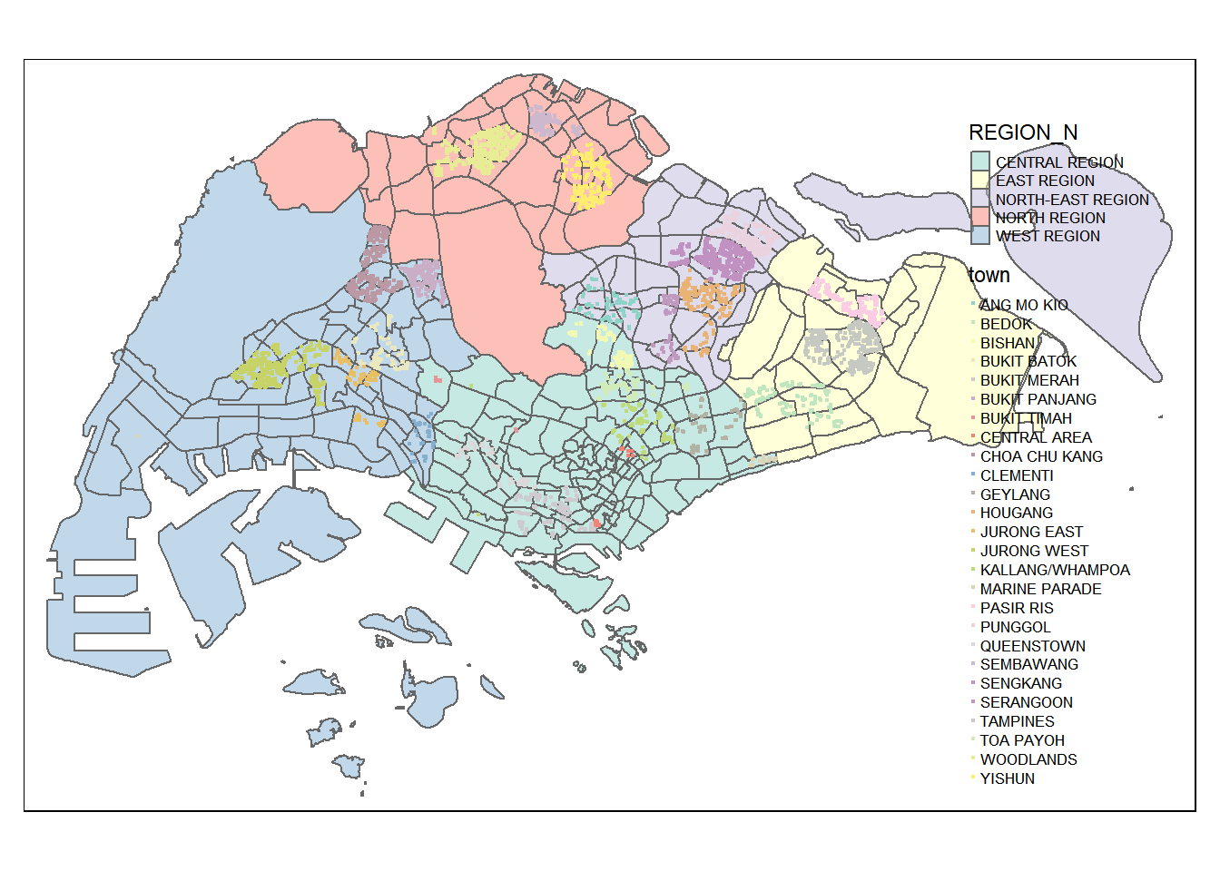
View Interactive Version of Map here! [20+mb]
Oddly, 27 Marine Cres appeared as a point on Sembcorp Marine Tuas Crescent and 54 Kent Rd somehow appeared as a point on 54J SOUTH BUONA VISTA ROAD KENT RIDGE HILL RESIDENCES. There are also some other differences, so let us now recode some of the addresses to get them to the right locations:
4.5.2.1 Fixing Data
We use mutate() to replace the existing addresses with more specific ones that we found on OneMap.
mod_hdb_resale_trans <- hdb_resale_trans %>% mutate(address = ifelse(address == "10 JLN BATU", "10 JALAN BATU DI TANJONG RHU", address)) %>% mutate(address = ifelse(address == "11 JLN BATU", "11 JALAN BATU DI TANJONG RHU", address)) %>% mutate(address = ifelse(address == "54 KENT RD", "54 KENT ROAD KENT VILLE", address)) %>% mutate(address = ifelse(address == "27 MARINE CRES", "27 MARINE CRESCENT MARINE CRESCENT VILLE", address))temp_hdb_resale_trans <- left_join(mod_hdb_resale_trans, coords_resale, by=c("address" = "address"))Lastly, we regenerate the list of unique Postal Codes to be geocoded.
addr_lst.resale_upd <- sort(unique(mod_hdb_resale_trans$address)) glimpse(addr_lst.resale_upd)chr [1:4037] "1 CHAI CHEE RD" "1 DELTA AVE" "1 EVERTON PK" "1 MARINE TER" ...We get the SVY21 X,Y coordinates using our get_coordinates() function
coords_resale_upd <- get_coordinates(addr_lst.resale_upd)Saving the DataFrame as .rds for future use to prevent rerunning get_coordinates() GET API everytime a render is run
write_rds(coords_resale_upd, "Take-Home_Ex03/rds/coords_resale_upd.rds")Load the DataFrame from .rds
coords_resale_upd <- read_rds("Take-Home_Ex03/rds/coords_resale_upd.rds")We left join the
hdb_hip_mup_trans_updmain table and coordinates and filter thexcolumn for any null valuestemp_hdb_resale_trans <- left_join(mod_hdb_resale_trans, coords_resale_upd, by=c("address" = "address")) filter(temp_hdb_resale_trans, is.na(x) == TRUE)# A tibble: 0 × 17 # ℹ 17 variables: month <chr>, town <chr>, flat_type <chr>, block <chr>, # street_name <chr>, storey_range <chr>, floor_area_sqm <dbl>, # flat_model <chr>, lease_commence_date <dbl>, remaining_lease <chr>, # resale_price <dbl>, address <chr>, remaining_lease_mths <dbl>, # age_of_unit_mths <dbl>, TYPE <chr>, x <chr>, y <chr>No null values found, we have completed this step!
hdb_resale_sf <- st_as_sf(temp_hdb_resale_trans, coords = c("x", "y"), crs = 3414)Generate external interactive map
tmap_mode("plot") hdb_plot2 <- tm_shape(mpsz) + tm_polygons("REGION_N", alpha = 0.5) + tm_shape(hdb_resale_sf) + tm_dots("town", popup.vars=c("block"="block", "street_name"="street_name", "flat_model" = "flat_model", "town" = "town", "resale_price" = "resale_price", "remaining_lease_mths", "remaining_lease_mths")) tmap_save(hdb_plot2, "thex03_hdbplot2.html")Static Plot
tmap_mode("plot") tm_shape(mpsz) + tm_polygons("REGION_N", alpha = 0.5) + tm_shape(hdb_resale_sf) + tm_dots("town", size = 0.05)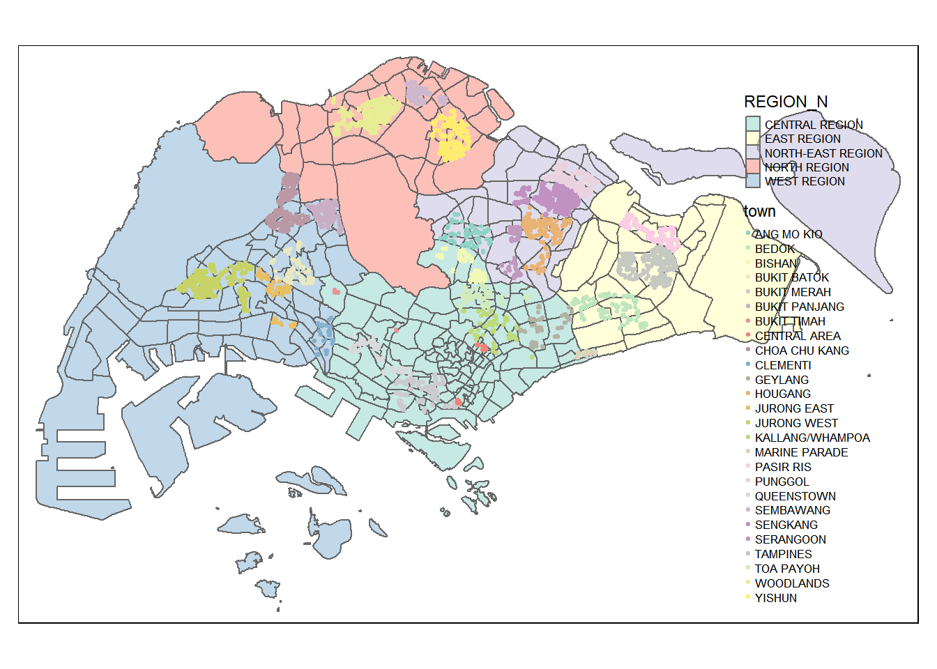
View Interactive Version of Map here! [20+mb]
Great! All the blocks looks to be plotted in the correct locations!
4.5.3 Shopping Malls
Merge Coordinate Data and Original Dataframe
temp_malls <- left_join(shopping_malls_raw, coords_malls, by=c("Mall_Name" = "address"))Check for
NAX/Y values and manually amend if requiredfilter(temp_malls, is.na(x) == TRUE)# A tibble: 0 × 4 # ℹ 4 variables: Mall_Name <chr>, Region <chr>, x <chr>, y <chr>No
NAvalues, great!Convert a DataFrame into a sf Object
We specify the SVY21 X and Y coordinates to be used as the coordinate geometry. The
crsspecified is3414which refers toSVY21.geo_malls <- st_as_sf(temp_malls, coords = c("x", "y"), crs = 3414)Plot a tmap and check if points are plotted in the correct regions
Now, we will plot an interactive tmap to check if our points are correct. We overlay the URA Master Plan Regions for a quick overlay to roughly check if the malls are located in the correct areas. Do note that mall region may differ from URA Planning Areas.
tmap_mode("view") tm_shape(mpsz) + tm_polygons("REGION_N", alpha = 0.5) + tm_shape(geo_malls) + tm_dots("Region", popup.vars=c("Mall_Name"="Mall_Name", "Region"="Region"), size = 0.05, palette = "Set2")Nice! All the malls seems to be in their right locations.
5 Preparing Locational Factors
From our list of locational factors, we can see that in general, we have two types of locational factors:
- Count of a factor within a certain radius
- Proximity of housing to a factor
We have created functions below that will prepare out data we require for our analysis.
5.1 Functions
5.1.1 Get Proximity Locational Factors
The get_prox() function below takes in an origin and destination dataframe and creates a distance matrix of origin and destination pairs based on st_distance(). Next, we use mutate and apply to locate the destination that is located the minimum distance away from the origin and save it to the corresponding row in origin_df under the PROX column. The 1 in apply is to apply the function row by row, which corresponds directly to the origin_df rows.
Next, we rename the columns based on whats specified by the input parameter and return the dataframe.
For the code below, we will use it to detect for 2 types of spatial types for destinations, Points and Linestring.
For our two linestring datasets, we know that there are:
- No HDBs within park boundaries
- No HDBs within Downtown Core
Hence, the following datasets will only need to factor distance to the boundary and there are no concerns that there are HDBs within those regions.
get_prox <- function(origin_df, dest_df, col_name){
# creates a matrix of distances
dist_matrix <- st_distance(origin_df, dest_df)
# find the nearest location_factor and create new data frame
near <- origin_df %>%
mutate(PROX = apply(dist_matrix, 1, function(x) min(x)) / 1000)
# rename column name according to input parameter
names(near)[names(near) == 'PROX'] <- col_name
# Return df
return(near)
}5.1.2 Get Num Within Locational Factors
The get_within() function below takes in an origin and destination dataframe and creates a distance matrix of origin and destination pairs based on st_distance().
Next, we use mutate and apply to obtain the sum of destinations that fits less than or equal to the threshold_dist specified and save the sum value to the corresponding row in origin_df under the PROX column. The 1 in apply is to apply the function row by row, which corresponds directly to the origin_df rows.
Next, we rename the columns based on whats specified by the input parameter and return the dataframe.
get_within <- function(origin_df, dest_df, threshold_dist, col_name){
# creates a matrix of distances
dist_matrix <- st_distance(origin_df, dest_df)
# count the number of location_factors within threshold_dist and create new data frame
wdist <- origin_df %>%
mutate(WITHIN_DT = apply(dist_matrix, 1, function(x) sum(x <= threshold_dist)))
# rename column name according to input parameter
names(wdist)[names(wdist) == 'WITHIN_DT'] <- col_name
# Return df
return(wdist)
}5.2 Generating Locational Factors and Saving Results
Using the code chunk below, we will generate the proximity to locational factors specified below:
geo_hdb_resale <- hdb_resale_sf
geo_hdb_resale <- get_prox(geo_hdb_resale, cbd_geom, "PROX_CBD")
geo_hdb_resale <- get_prox(geo_hdb_resale, geo_eldercare, "PROX_ELDER")
geo_hdb_resale <- get_prox(geo_hdb_resale, geo_hawker, "PROX_HAWKER")
geo_hdb_resale <- get_prox(geo_hdb_resale, geo_mrt_existing, "PROX_MRT_E")
geo_hdb_resale <- get_prox(geo_hdb_resale, geo_parks, "PROX_PARK")
geo_hdb_resale <- get_prox(geo_hdb_resale, geo_top_schools, "PROX_TOP_SCH")
geo_hdb_resale <- get_prox(geo_hdb_resale, geo_malls, "PROX_MALL")
geo_hdb_resale <- get_prox(geo_hdb_resale, geo_supermarkets, "PROX_SUPMKT")
geo_hdb_resale <- get_prox(geo_hdb_resale, geo_rail_mrt_above, "PROX_TRK_MRT")
geo_hdb_resale <- get_prox(geo_hdb_resale, geo_rail_lrt_above, "PROX_TRK_LRT")Now, using the code chunk below, we will obtain the count of location factors specified:
geo_hdb_resale <- get_within(geo_hdb_resale, geo_childcare, 350, "NUM_350_CHILD")
geo_hdb_resale <- get_within(geo_hdb_resale, geo_kindergartens, 350, "NUM_350_KINDER")
geo_hdb_resale <- get_within(geo_hdb_resale, geo_bus_stop, 350, "NUM_350_BUS")
geo_hdb_resale <- get_within(geo_hdb_resale, geo_schools, 1000, "NUM_1000_SCH")
geo_hdb_resale <- get_within(geo_hdb_resale, geo_mrt_future, 800, "NUM_800_MRT_F")
geo_hdb_resale <- get_within(geo_hdb_resale, geo_lrt, 350, "NUM_350_LRT")To prevent running the code above again on every render, we will save the results to a RDS file. We will use the read script to read the file without having to rerun the processing on every render.
write_rds(geo_hdb_resale, "Take-Home_Ex03/rds/geo_hdb_resale.rds")geo_hdb_resale <- read_rds("Take-Home_Ex03/rds/geo_hdb_resale.rds")6 Preparing Structural Factors
Looking at the list of structural factors, there are some factors that requires further processing. These strucutral factors are listed in the table below.
| dName of Structural Factor | Data Type | Remarks |
|---|---|---|
| Area of Unit | Numerical | |
| Floor Level | Categorical | Requires recoding of values |
| Remaining Lease | Numerical | Data has been processed to numerical readable values in months in Transforming Aspatial Data - Create New Columns with Values |
| Age of the unit | Numerical | |
| Main Upgrading Program (MUP) Completed | Categorical | Requires one-hot encoding |
| Apartment Model | Categorical | This data has to be derived and standardised from flat_model |
| Apartment Multi-story | Categorical | This data has to be derived and standardised from flat_model |
Now, let us first look at the floor levels.
storeys <- sort(unique(geo_hdb_resale$storey_range))
storeys [1] "01 TO 03" "04 TO 06" "07 TO 09" "10 TO 12" "13 TO 15" "16 TO 18"
[7] "19 TO 21" "22 TO 24" "25 TO 27" "28 TO 30" "31 TO 33" "34 TO 36"
[13] "37 TO 39" "40 TO 42" "43 TO 45" "46 TO 48" "49 TO 51"From the unique values obtained above, we can see that story range is provided as a categorical range of every three floors. In the data above, we can see that there are 17 storey range categories.
Let us recode the categorical naming to numerical values by assigning 1 to the first range 01 TO 03 and 17 to the last range 49 TO 51.
storey_order <- 1:length(storeys)
storey_range_order <- data.frame(storeys, storey_order)
storey_range_order storeys storey_order
1 01 TO 03 1
2 04 TO 06 2
3 07 TO 09 3
4 10 TO 12 4
5 13 TO 15 5
6 16 TO 18 6
7 19 TO 21 7
8 22 TO 24 8
9 25 TO 27 9
10 28 TO 30 10
11 31 TO 33 11
12 34 TO 36 12
13 37 TO 39 13
14 40 TO 42 14
15 43 TO 45 15
16 46 TO 48 16
17 49 TO 51 17From our data frame above, we have obtained the storey ranges and storey_order. Using the code below, we will use left_join to join storey_order to the main geo_hdb_resale dataframe.
geo_hdb_resale <- left_join(geo_hdb_resale, storey_range_order, by = c("storey_range" = "storeys"))There we go, we have combined the recorded storey range values as storey_order.
6.1 HDB Apartment Model and Multi-storey
Not all HDB Apartments are built the same, there are different HDB Models and some HDB units are multi-storey. Let us explore what kinds of models do we have in our dataset:
unique(geo_hdb_resale$flat_model) [1] "Improved" "Standard" "Model A"
[4] "DBSS" "Adjoined flat" "Premium Apartment"
[7] "Model A-Maisonette" "Type S2" "Improved-Maisonette"
[10] "Premium Apartment Loft" "3Gen" From our data above, we can see that we have 11 distinct categories of HDB Apartment Types. Some of these terminologies changed over time and may refer to the configuration or whether the apartments came with furnishings.
Let use understand what some of the terms mean:
Design Build Sell Scheme (DBSS) flats may call for a higher value than regular HDB flats as they are designed, build and sold by 3rd party developers although they are still HDB Flats. They are supposed to be better than premium flats
Premium flats which come with pre-installed fittings and furnishings over standard apartments which comes with none
Standard flats are opposite of premium, they don’t come with furnishings or fittings
Maisonette / Loft comes with a second floor of apartment space
3Gen is a new type of single-key unit with additional bedroom and bathroom for grandparents to live in
Adjoined flats are units where two HDB units are combined (may or may not have 2 front doors)
Type S2 are types assigned to 5-room units in The Pinnacle at Duxton
Let us recode them so that the model can generalise better.
| Original Values | Recoded Values (model_<valuename>) | Recoded Values (multistorey) |
|---|---|---|
| Improved | Standard = 1 | 0 |
| Standard | Standard = 1 | 0 |
| DBSS | DBSS = 1 | 0 |
| Model A | Standard = 1 | 0 |
| Adjoined flat | Adjoined = 1 | 0 |
| Premium Apartment | Premium = 1 | 0 |
| Type S2 | S2 = 1 | 0 |
| Model A-Maisonette | Standard = 1 | 1 |
| Premium Apartment Loft | Premium = 1 | 1 |
| Improved - Maisonette | Standard = 1 | 1 |
| 3Gen | 3Gen = 1 | 0 |
## Create Multistorey Columns
Using the code chunk below, we will check if the flat_model corresponds to the following types, if it is, we code the value in the multistorey as 1. Else, 0 is assigned.
geo_hdb_resale <- geo_hdb_resale %>% mutate(multistorey = ifelse(flat_model %in% c("Improved-Maisonette", "Model A-Maisonette", "Premium Apartment Loft"), 1, 0 ))geo_hdb_resale <- geo_hdb_resale %>% mutate(model_standard = ifelse(flat_model %in% c("Improved", "Standard", "Model A", "Model A-Maisonette", "Improved-Maisonette"), 1, 0))
geo_hdb_resale <- geo_hdb_resale %>% mutate(model_premium = ifelse(flat_model %in% c("Premium Apartment", "Premium Apartment Loft"), 1, 0))
geo_hdb_resale <- geo_hdb_resale %>% mutate(model_dbss = ifelse(flat_model %in% c("DBSS"), 1, 0))
geo_hdb_resale <- geo_hdb_resale %>% mutate(model_adjoined = ifelse(flat_model %in% c("Adjoined flat"), 1, 0))
geo_hdb_resale <- geo_hdb_resale %>% mutate(model_3gen = ifelse(flat_model %in% c("3Gen"), 1, 0))
geo_hdb_resale <- geo_hdb_resale %>% mutate(model_s2 = ifelse(flat_model %in% c("Type S2"), 1, 0))Nice, we have completed our recoding, let us view a snippet of our data
glimpse(geo_hdb_resale)Rows: 15,549
Columns: 40
$ month <chr> "2021-01", "2021-01", "2021-01", "2021-01", "2021…
$ town <chr> "ANG MO KIO", "ANG MO KIO", "ANG MO KIO", "ANG MO…
$ flat_type <chr> "5 ROOM", "5 ROOM", "5 ROOM", "5 ROOM", "5 ROOM",…
$ block <chr> "551", "305", "520", "253", "423", "617", "315A",…
$ street_name <chr> "ANG MO KIO AVE 10", "ANG MO KIO AVE 1", "ANG MO …
$ storey_range <chr> "01 TO 03", "13 TO 15", "16 TO 18", "07 TO 09", "…
$ floor_area_sqm <dbl> 118, 123, 118, 128, 133, 133, 110, 110, 110, 112,…
$ flat_model <chr> "Improved", "Standard", "Improved", "Improved", "…
$ lease_commence_date <dbl> 1981, 1977, 1980, 1996, 1993, 1996, 2006, 2002, 2…
$ remaining_lease <chr> "59 years 01 month", "55 years 07 months", "58 ye…
$ resale_price <dbl> 483000, 590000, 629000, 670000, 680000, 760000, 7…
$ address <chr> "551 ANG MO KIO AVE 10", "305 ANG MO KIO AVE 1", …
$ remaining_lease_mths <dbl> 709, 667, 704, 891, 855, 894, 1012, 971, 1012, 10…
$ age_of_unit_mths <dbl> 479, 521, 484, 297, 333, 294, 176, 217, 176, 113,…
$ TYPE <chr> "HIP", "MUP", "HIP", NA, "MUP", NA, NA, NA, NA, N…
$ geometry <POINT [m]> POINT (30820.82 39547.58), POINT (29412.84 …
$ PROX_CBD <dbl> 7.737105, 7.028289, 7.784321, 7.658682, 7.268078,…
$ PROX_ELDER <dbl> 1.0646617, 0.1908834, 0.7891907, 0.1476040, 0.441…
$ PROX_HAWKER <dbl> 0.4828156, 0.3317637, 0.3792242, 0.5884497, 0.512…
$ PROX_MRT_E <dbl> 1.0208473, 0.6367554, 0.4337494, 0.3761649, 0.154…
$ PROX_PARK <dbl> 0.68961631, 0.24220780, 0.17955893, 0.24017236, 0…
$ PROX_TOP_SCH <dbl> 1.7671659, 1.2666115, 1.8845549, 0.5556902, 1.777…
$ PROX_MALL <dbl> 1.2132867, 0.4568608, 0.3929283, 1.2859841, 0.373…
$ PROX_SUPMKT <dbl> 0.41991387, 0.24554343, 0.31805791, 0.31357577, 0…
$ PROX_TRK_MRT <dbl> 1.0812150, 0.5418813, 0.2971287, 1.5706019, 0.150…
$ PROX_TRK_LRT <dbl> 2.779188, 4.408028, 3.462856, 5.249395, 3.729856,…
$ NUM_350_CHILD <int> 3, 6, 4, 3, 3, 3, 5, 2, 6, 5, 6, 5, 5, 5, 1, 5, 3…
$ NUM_350_KINDER <int> 1, 1, 1, 1, 1, 1, 1, 0, 1, 1, 1, 1, 1, 0, 0, 0, 1…
$ NUM_350_BUS <int> 2, 8, 6, 11, 6, 8, 4, 9, 5, 9, 7, 9, 9, 11, 5, 6,…
$ NUM_1000_SCH <int> 1, 3, 3, 3, 3, 4, 2, 3, 2, 2, 2, 2, 2, 4, 2, 3, 3…
$ NUM_800_MRT_F <int> 1, 1, 0, 0, 0, 0, 1, 0, 1, 0, 0, 0, 0, 0, 0, 1, 0…
$ NUM_350_LRT <int> 0, 0, 0, 0, 0, 0, 0, 0, 0, 0, 0, 0, 0, 0, 0, 0, 0…
$ storey_order <int> 1, 5, 6, 3, 1, 5, 8, 5, 6, 6, 5, 5, 8, 2, 2, 3, 1…
$ multistorey <dbl> 0, 0, 0, 0, 0, 0, 0, 0, 0, 0, 0, 0, 0, 0, 0, 0, 0…
$ model_standard <dbl> 1, 1, 1, 1, 1, 1, 1, 1, 1, 0, 0, 0, 0, 1, 1, 1, 1…
$ model_premium <dbl> 0, 0, 0, 0, 0, 0, 0, 0, 0, 0, 0, 0, 0, 0, 0, 0, 0…
$ model_dbss <dbl> 0, 0, 0, 0, 0, 0, 0, 0, 0, 1, 1, 1, 1, 0, 0, 0, 0…
$ model_adjoined <dbl> 0, 0, 0, 0, 0, 0, 0, 0, 0, 0, 0, 0, 0, 0, 0, 0, 0…
$ model_3gen <dbl> 0, 0, 0, 0, 0, 0, 0, 0, 0, 0, 0, 0, 0, 0, 0, 0, 0…
$ model_s2 <dbl> 0, 0, 0, 0, 0, 0, 0, 0, 0, 0, 0, 0, 0, 0, 0, 0, 0…6.2 HDB HIP MUP
Similarly for HIP MUP data, since there are all coded as HIP or MUP or NA cateogrical values, we need to convert them to numbers so that the model will be able to build.
In this case, we will create two new columns, HIP and MUP to track which kind of upgrading project has been done on the unit.
Using the code chunk, we will recode the respective values into the respective columns as 1 (true) or 0 (false).
geo_hdb_resale <- geo_hdb_resale %>% mutate(hip = ifelse(is.na(TYPE), 0, ifelse(TYPE == "HIP", 1, 0)))
geo_hdb_resale <- geo_hdb_resale %>% mutate(mup = ifelse(is.na(TYPE), 0, ifelse(TYPE == "MUP", 1, 0)))The manipulation is complete, let us glimpse the values.
glimpse(geo_hdb_resale)Rows: 15,549
Columns: 42
$ month <chr> "2021-01", "2021-01", "2021-01", "2021-01", "2021…
$ town <chr> "ANG MO KIO", "ANG MO KIO", "ANG MO KIO", "ANG MO…
$ flat_type <chr> "5 ROOM", "5 ROOM", "5 ROOM", "5 ROOM", "5 ROOM",…
$ block <chr> "551", "305", "520", "253", "423", "617", "315A",…
$ street_name <chr> "ANG MO KIO AVE 10", "ANG MO KIO AVE 1", "ANG MO …
$ storey_range <chr> "01 TO 03", "13 TO 15", "16 TO 18", "07 TO 09", "…
$ floor_area_sqm <dbl> 118, 123, 118, 128, 133, 133, 110, 110, 110, 112,…
$ flat_model <chr> "Improved", "Standard", "Improved", "Improved", "…
$ lease_commence_date <dbl> 1981, 1977, 1980, 1996, 1993, 1996, 2006, 2002, 2…
$ remaining_lease <chr> "59 years 01 month", "55 years 07 months", "58 ye…
$ resale_price <dbl> 483000, 590000, 629000, 670000, 680000, 760000, 7…
$ address <chr> "551 ANG MO KIO AVE 10", "305 ANG MO KIO AVE 1", …
$ remaining_lease_mths <dbl> 709, 667, 704, 891, 855, 894, 1012, 971, 1012, 10…
$ age_of_unit_mths <dbl> 479, 521, 484, 297, 333, 294, 176, 217, 176, 113,…
$ TYPE <chr> "HIP", "MUP", "HIP", NA, "MUP", NA, NA, NA, NA, N…
$ geometry <POINT [m]> POINT (30820.82 39547.58), POINT (29412.84 …
$ PROX_CBD <dbl> 7.737105, 7.028289, 7.784321, 7.658682, 7.268078,…
$ PROX_ELDER <dbl> 1.0646617, 0.1908834, 0.7891907, 0.1476040, 0.441…
$ PROX_HAWKER <dbl> 0.4828156, 0.3317637, 0.3792242, 0.5884497, 0.512…
$ PROX_MRT_E <dbl> 1.0208473, 0.6367554, 0.4337494, 0.3761649, 0.154…
$ PROX_PARK <dbl> 0.68961631, 0.24220780, 0.17955893, 0.24017236, 0…
$ PROX_TOP_SCH <dbl> 1.7671659, 1.2666115, 1.8845549, 0.5556902, 1.777…
$ PROX_MALL <dbl> 1.2132867, 0.4568608, 0.3929283, 1.2859841, 0.373…
$ PROX_SUPMKT <dbl> 0.41991387, 0.24554343, 0.31805791, 0.31357577, 0…
$ PROX_TRK_MRT <dbl> 1.0812150, 0.5418813, 0.2971287, 1.5706019, 0.150…
$ PROX_TRK_LRT <dbl> 2.779188, 4.408028, 3.462856, 5.249395, 3.729856,…
$ NUM_350_CHILD <int> 3, 6, 4, 3, 3, 3, 5, 2, 6, 5, 6, 5, 5, 5, 1, 5, 3…
$ NUM_350_KINDER <int> 1, 1, 1, 1, 1, 1, 1, 0, 1, 1, 1, 1, 1, 0, 0, 0, 1…
$ NUM_350_BUS <int> 2, 8, 6, 11, 6, 8, 4, 9, 5, 9, 7, 9, 9, 11, 5, 6,…
$ NUM_1000_SCH <int> 1, 3, 3, 3, 3, 4, 2, 3, 2, 2, 2, 2, 2, 4, 2, 3, 3…
$ NUM_800_MRT_F <int> 1, 1, 0, 0, 0, 0, 1, 0, 1, 0, 0, 0, 0, 0, 0, 1, 0…
$ NUM_350_LRT <int> 0, 0, 0, 0, 0, 0, 0, 0, 0, 0, 0, 0, 0, 0, 0, 0, 0…
$ storey_order <int> 1, 5, 6, 3, 1, 5, 8, 5, 6, 6, 5, 5, 8, 2, 2, 3, 1…
$ multistorey <dbl> 0, 0, 0, 0, 0, 0, 0, 0, 0, 0, 0, 0, 0, 0, 0, 0, 0…
$ model_standard <dbl> 1, 1, 1, 1, 1, 1, 1, 1, 1, 0, 0, 0, 0, 1, 1, 1, 1…
$ model_premium <dbl> 0, 0, 0, 0, 0, 0, 0, 0, 0, 0, 0, 0, 0, 0, 0, 0, 0…
$ model_dbss <dbl> 0, 0, 0, 0, 0, 0, 0, 0, 0, 1, 1, 1, 1, 0, 0, 0, 0…
$ model_adjoined <dbl> 0, 0, 0, 0, 0, 0, 0, 0, 0, 0, 0, 0, 0, 0, 0, 0, 0…
$ model_3gen <dbl> 0, 0, 0, 0, 0, 0, 0, 0, 0, 0, 0, 0, 0, 0, 0, 0, 0…
$ model_s2 <dbl> 0, 0, 0, 0, 0, 0, 0, 0, 0, 0, 0, 0, 0, 0, 0, 0, 0…
$ hip <dbl> 1, 0, 1, 0, 0, 0, 0, 0, 0, 0, 0, 0, 0, 0, 0, 0, 0…
$ mup <dbl> 0, 1, 0, 0, 1, 0, 0, 0, 0, 0, 0, 0, 0, 1, 0, 1, 0…6.3 RDS Scripts and Preparing for EDA
We will now save our prepared HDB Resale dataset and mpsz to a RDS file and clear all variables to free up the memory before reloading the dataset as final_resale.
The rm(list=ls()) function will clear all variables
write_rds(geo_hdb_resale,"Take-Home_Ex03/rds/final_resale.rds")
write_rds(mpsz,"Take-Home_Ex03/rds/mpsz.rds")rm(list=ls())final_resale <- read_rds("Take-Home_Ex03/rds/final_resale.rds")
mpsz <- read_rds("Take-Home_Ex03/rds/mpsz.rds")7 Exploratory Data Analysis
Now, we can perform EDA on our prepared dataset geo_hdb_resale to better understand our dataset.
glimpse(final_resale)Rows: 15,549
Columns: 42
$ month <chr> "2021-01", "2021-01", "2021-01", "2021-01", "2021…
$ town <chr> "ANG MO KIO", "ANG MO KIO", "ANG MO KIO", "ANG MO…
$ flat_type <chr> "5 ROOM", "5 ROOM", "5 ROOM", "5 ROOM", "5 ROOM",…
$ block <chr> "551", "305", "520", "253", "423", "617", "315A",…
$ street_name <chr> "ANG MO KIO AVE 10", "ANG MO KIO AVE 1", "ANG MO …
$ storey_range <chr> "01 TO 03", "13 TO 15", "16 TO 18", "07 TO 09", "…
$ floor_area_sqm <dbl> 118, 123, 118, 128, 133, 133, 110, 110, 110, 112,…
$ flat_model <chr> "Improved", "Standard", "Improved", "Improved", "…
$ lease_commence_date <dbl> 1981, 1977, 1980, 1996, 1993, 1996, 2006, 2002, 2…
$ remaining_lease <chr> "59 years 01 month", "55 years 07 months", "58 ye…
$ resale_price <dbl> 483000, 590000, 629000, 670000, 680000, 760000, 7…
$ address <chr> "551 ANG MO KIO AVE 10", "305 ANG MO KIO AVE 1", …
$ remaining_lease_mths <dbl> 709, 667, 704, 891, 855, 894, 1012, 971, 1012, 10…
$ age_of_unit_mths <dbl> 479, 521, 484, 297, 333, 294, 176, 217, 176, 113,…
$ TYPE <chr> "HIP", "MUP", "HIP", NA, "MUP", NA, NA, NA, NA, N…
$ geometry <POINT [m]> POINT (30820.82 39547.58), POINT (29412.84 …
$ PROX_CBD <dbl> 7.737105, 7.028289, 7.784321, 7.658682, 7.268078,…
$ PROX_ELDER <dbl> 1.0646617, 0.1908834, 0.7891907, 0.1476040, 0.441…
$ PROX_HAWKER <dbl> 0.4828156, 0.3317637, 0.3792242, 0.5884497, 0.512…
$ PROX_MRT_E <dbl> 1.0208473, 0.6367554, 0.4337494, 0.3761649, 0.154…
$ PROX_PARK <dbl> 0.68961631, 0.24220780, 0.17955893, 0.24017236, 0…
$ PROX_TOP_SCH <dbl> 1.7671659, 1.2666115, 1.8845549, 0.5556902, 1.777…
$ PROX_MALL <dbl> 1.2132867, 0.4568608, 0.3929283, 1.2859841, 0.373…
$ PROX_SUPMKT <dbl> 0.41991387, 0.24554343, 0.31805791, 0.31357577, 0…
$ PROX_TRK_MRT <dbl> 1.0812150, 0.5418813, 0.2971287, 1.5706019, 0.150…
$ PROX_TRK_LRT <dbl> 2.779188, 4.408028, 3.462856, 5.249395, 3.729856,…
$ NUM_350_CHILD <int> 3, 6, 4, 3, 3, 3, 5, 2, 6, 5, 6, 5, 5, 5, 1, 5, 3…
$ NUM_350_KINDER <int> 1, 1, 1, 1, 1, 1, 1, 0, 1, 1, 1, 1, 1, 0, 0, 0, 1…
$ NUM_350_BUS <int> 2, 8, 6, 11, 6, 8, 4, 9, 5, 9, 7, 9, 9, 11, 5, 6,…
$ NUM_1000_SCH <int> 1, 3, 3, 3, 3, 4, 2, 3, 2, 2, 2, 2, 2, 4, 2, 3, 3…
$ NUM_800_MRT_F <int> 1, 1, 0, 0, 0, 0, 1, 0, 1, 0, 0, 0, 0, 0, 0, 1, 0…
$ NUM_350_LRT <int> 0, 0, 0, 0, 0, 0, 0, 0, 0, 0, 0, 0, 0, 0, 0, 0, 0…
$ storey_order <int> 1, 5, 6, 3, 1, 5, 8, 5, 6, 6, 5, 5, 8, 2, 2, 3, 1…
$ multistorey <dbl> 0, 0, 0, 0, 0, 0, 0, 0, 0, 0, 0, 0, 0, 0, 0, 0, 0…
$ model_standard <dbl> 1, 1, 1, 1, 1, 1, 1, 1, 1, 0, 0, 0, 0, 1, 1, 1, 1…
$ model_premium <dbl> 0, 0, 0, 0, 0, 0, 0, 0, 0, 0, 0, 0, 0, 0, 0, 0, 0…
$ model_dbss <dbl> 0, 0, 0, 0, 0, 0, 0, 0, 0, 1, 1, 1, 1, 0, 0, 0, 0…
$ model_adjoined <dbl> 0, 0, 0, 0, 0, 0, 0, 0, 0, 0, 0, 0, 0, 0, 0, 0, 0…
$ model_3gen <dbl> 0, 0, 0, 0, 0, 0, 0, 0, 0, 0, 0, 0, 0, 0, 0, 0, 0…
$ model_s2 <dbl> 0, 0, 0, 0, 0, 0, 0, 0, 0, 0, 0, 0, 0, 0, 0, 0, 0…
$ hip <dbl> 1, 0, 1, 0, 0, 0, 0, 0, 0, 0, 0, 0, 0, 0, 0, 0, 0…
$ mup <dbl> 0, 1, 0, 0, 1, 0, 0, 0, 0, 0, 0, 0, 0, 1, 0, 1, 0…7.1 Removing Columns Not Required For Analysis
Firstly, let us remove the columns that are not required for further analysis to save on memory space.
To do this, we use the select() function and indicate the columns we want to remove by having the prefix-
final_resale <- select(final_resale, c(-flat_type,-storey_range,-flat_model, -lease_commence_date, -address, -TYPE, -remaining_lease))Now, let us view the columns remaining.
glimpse(final_resale)Rows: 15,549
Columns: 35
$ month <chr> "2021-01", "2021-01", "2021-01", "2021-01", "2021…
$ town <chr> "ANG MO KIO", "ANG MO KIO", "ANG MO KIO", "ANG MO…
$ block <chr> "551", "305", "520", "253", "423", "617", "315A",…
$ street_name <chr> "ANG MO KIO AVE 10", "ANG MO KIO AVE 1", "ANG MO …
$ floor_area_sqm <dbl> 118, 123, 118, 128, 133, 133, 110, 110, 110, 112,…
$ resale_price <dbl> 483000, 590000, 629000, 670000, 680000, 760000, 7…
$ remaining_lease_mths <dbl> 709, 667, 704, 891, 855, 894, 1012, 971, 1012, 10…
$ age_of_unit_mths <dbl> 479, 521, 484, 297, 333, 294, 176, 217, 176, 113,…
$ geometry <POINT [m]> POINT (30820.82 39547.58), POINT (29412.84 …
$ PROX_CBD <dbl> 7.737105, 7.028289, 7.784321, 7.658682, 7.268078,…
$ PROX_ELDER <dbl> 1.0646617, 0.1908834, 0.7891907, 0.1476040, 0.441…
$ PROX_HAWKER <dbl> 0.4828156, 0.3317637, 0.3792242, 0.5884497, 0.512…
$ PROX_MRT_E <dbl> 1.0208473, 0.6367554, 0.4337494, 0.3761649, 0.154…
$ PROX_PARK <dbl> 0.68961631, 0.24220780, 0.17955893, 0.24017236, 0…
$ PROX_TOP_SCH <dbl> 1.7671659, 1.2666115, 1.8845549, 0.5556902, 1.777…
$ PROX_MALL <dbl> 1.2132867, 0.4568608, 0.3929283, 1.2859841, 0.373…
$ PROX_SUPMKT <dbl> 0.41991387, 0.24554343, 0.31805791, 0.31357577, 0…
$ PROX_TRK_MRT <dbl> 1.0812150, 0.5418813, 0.2971287, 1.5706019, 0.150…
$ PROX_TRK_LRT <dbl> 2.779188, 4.408028, 3.462856, 5.249395, 3.729856,…
$ NUM_350_CHILD <int> 3, 6, 4, 3, 3, 3, 5, 2, 6, 5, 6, 5, 5, 5, 1, 5, 3…
$ NUM_350_KINDER <int> 1, 1, 1, 1, 1, 1, 1, 0, 1, 1, 1, 1, 1, 0, 0, 0, 1…
$ NUM_350_BUS <int> 2, 8, 6, 11, 6, 8, 4, 9, 5, 9, 7, 9, 9, 11, 5, 6,…
$ NUM_1000_SCH <int> 1, 3, 3, 3, 3, 4, 2, 3, 2, 2, 2, 2, 2, 4, 2, 3, 3…
$ NUM_800_MRT_F <int> 1, 1, 0, 0, 0, 0, 1, 0, 1, 0, 0, 0, 0, 0, 0, 1, 0…
$ NUM_350_LRT <int> 0, 0, 0, 0, 0, 0, 0, 0, 0, 0, 0, 0, 0, 0, 0, 0, 0…
$ storey_order <int> 1, 5, 6, 3, 1, 5, 8, 5, 6, 6, 5, 5, 8, 2, 2, 3, 1…
$ multistorey <dbl> 0, 0, 0, 0, 0, 0, 0, 0, 0, 0, 0, 0, 0, 0, 0, 0, 0…
$ model_standard <dbl> 1, 1, 1, 1, 1, 1, 1, 1, 1, 0, 0, 0, 0, 1, 1, 1, 1…
$ model_premium <dbl> 0, 0, 0, 0, 0, 0, 0, 0, 0, 0, 0, 0, 0, 0, 0, 0, 0…
$ model_dbss <dbl> 0, 0, 0, 0, 0, 0, 0, 0, 0, 1, 1, 1, 1, 0, 0, 0, 0…
$ model_adjoined <dbl> 0, 0, 0, 0, 0, 0, 0, 0, 0, 0, 0, 0, 0, 0, 0, 0, 0…
$ model_3gen <dbl> 0, 0, 0, 0, 0, 0, 0, 0, 0, 0, 0, 0, 0, 0, 0, 0, 0…
$ model_s2 <dbl> 0, 0, 0, 0, 0, 0, 0, 0, 0, 0, 0, 0, 0, 0, 0, 0, 0…
$ hip <dbl> 1, 0, 1, 0, 0, 0, 0, 0, 0, 0, 0, 0, 0, 0, 0, 0, 0…
$ mup <dbl> 0, 1, 0, 0, 1, 0, 0, 0, 0, 0, 0, 0, 0, 1, 0, 1, 0…7.2 Understanding Resale Prices
Now, let us plot a histogram to understand the pricing of 5-Room resale flats between Jan 2020 to Feb 2023.
ggplot(final_resale, aes(x=resale_price)) +
geom_histogram(bins = 20, color = "black", fill = "lightblue")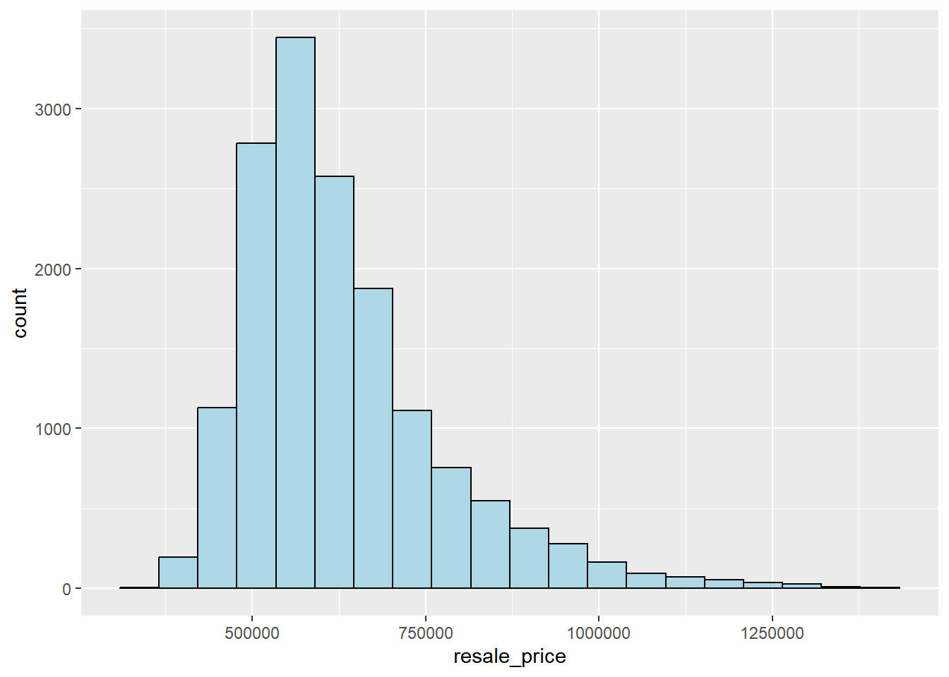
From our graph above, we can see that:
Right-skewed distribution of resale_prices
Most resale HDBs are transacted near the $500,000 range.
Outliers are seen where HDB prices are transacted near $1 million or more
In this scenerio, while we can take log of resale_price, we will not perform the transformation to make it a normal distribution as:
resale_priceis the value to be predicted, we do not want to predict the log ofresale_price- Using the log of
resale_pricewill cause it to have a high correlation with actualresale_price
7.3 Understanding Structural Factors
To understand more about the structural factors regarding 5-room HDB resale units of our prepared datasets, we can plot the graphs below.
Using the code chunk below, we prepare the variables to plot according to numerical (s_factor) and categorical data (s_factor_cat).
s_factor <- c("floor_area_sqm", "storey_order", "remaining_lease_mths", "age_of_unit_mths")
s_factor_cat <- c("mup", "hip", "model_standard", "model_premium", "model_dbss", "model_adjoined", "model_3gen", "model_s2", "multistorey")The code chunk below also defines the methods to plot each graph, numerical and categorical data. It will iterate the list data in s_factor and s_factor_cat respectively to seperate plots. The graph data is saved into lists s_factor_hist_list and s_factor_hist_list_cat.
s_factor_hist_list <- c()
for (i in 1:length(s_factor)) {
hist_plot <- ggplot(final_resale, aes_string(x = s_factor[[i]])) +
geom_histogram(color="black", fill = "lightblue") +
labs(title = s_factor[[i]]) +
theme(plot.title = element_text(size = 10),
axis.title = element_blank())
s_factor_hist_list[[i]] <- hist_plot
}
s_factor_hist_list_cat <- c()
for (i in 1:length(s_factor_cat)) {
hist_plot <- ggplot(final_resale, aes_string(x = s_factor_cat[[i]])) +
geom_histogram(bins = 2, color="black", fill = "lightblue") +
labs(title = s_factor_cat[[i]]) +
theme(plot.title = element_text(size = 10),
axis.title = element_blank())
s_factor_hist_list_cat[[i]] <- hist_plot
}Lastly with the list data, we can plot them using ggarrange() with our desired row and columns below.
Numerical Data:
ggarrange(plotlist = s_factor_hist_list,
ncol = 2,
nrow = 2)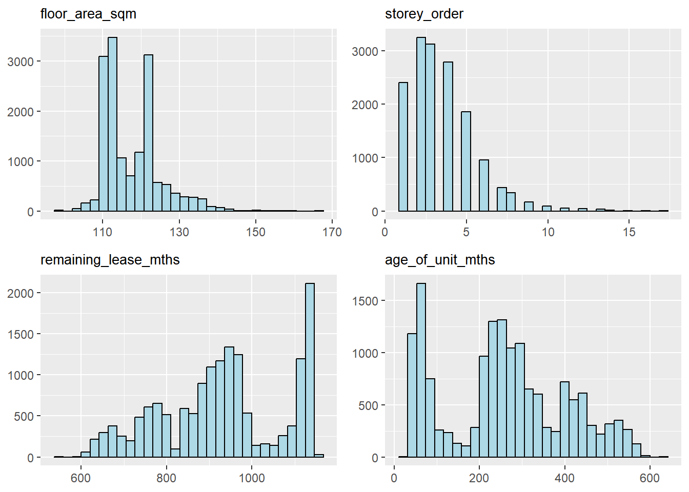
From the numerical plots above we can see that:
floor_area_sqmis right skewed, most units has a floor area of aprox. 110sqm to 120sqm. There are outlier 5-room units with sizes of about 150sqm.store_orderis right skewed. This shows that most units sold are mostly low floor units of with the most at aboutstorey_order= 3, meaning 3*3 = 9 to 11 storeys. This is so as many older HDBs are shorter in height and only newer HDBs exceed 16 storeys. Some estates like Punggol and Sengkang also has height restrictions that mostly cap new HDBs at about 16 storeys.remaining_lease_mthsis left skewed, topping at at the rightmost part of the chart. It could be seen as most homeowners trying to sell their houses after the 5-year Minimum Occupation Period. As the house is older in length, the amount of apartment sales reduces. The next peak in sales after the minimum 5-year Minimum Occupation Period is approximately 20-Years.age_of_unit_mthsis right skewed and a inverse relationship toremaining_lease_mths
Categorical Data:
ggarrange(plotlist = s_factor_hist_list_cat,
ncol = 3,
nrow = 3)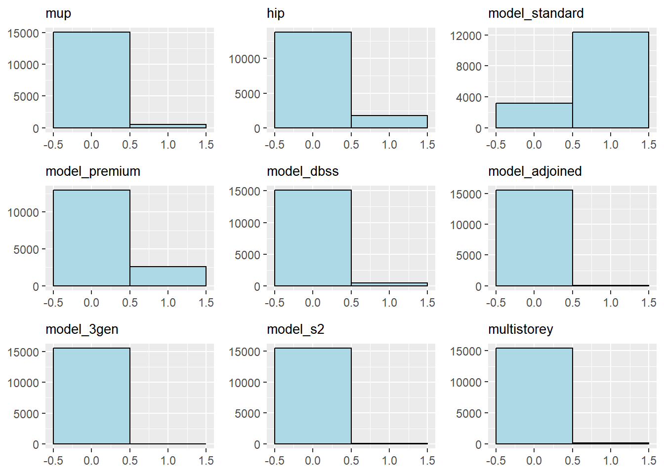
Very little flats received the Main Upgrading Programme
About 2000 flats received the Home Improvement Porgramme (successor to the Main Upgrading Programme)
Standard Flat Models are approximately the inverse of Premium Flat Models
There is very little DBSS Model Units
Adjoined, S2 (Painnacle at Duxton), 3 Generation and Multistorey resale units are extremely rare
7.4 Understanding Locational Factors
Similarly to structural factors, we will plot the locational factors to see its trends.
l_factor <- c("PROX_CBD", "PROX_ELDER", "PROX_HAWKER", "PROX_MRT_E",
"PROX_PARK", "PROX_TOP_SCH", "PROX_MALL", "PROX_SUPMKT",
"PROX_TRK_MRT", "PROX_TRK_LRT", "NUM_350_CHILD", "NUM_350_BUS", "NUM_1000_SCH", "NUM_800_MRT_F", "NUM_350_LRT")
l_factor_hist_list <- c()
for (i in 1:length(l_factor)) {
hist_plot <- ggplot(final_resale, aes_string(x = l_factor[[i]])) +
geom_histogram(color="black", fill = "lightblue") +
labs(title = l_factor[[i]]) +
theme(plot.title = element_text(size = 10),
axis.title = element_blank())
l_factor_hist_list[[i]] <- hist_plot
}ggarrange(plotlist = l_factor_hist_list,
ncol = 2,
nrow = 2)$`1`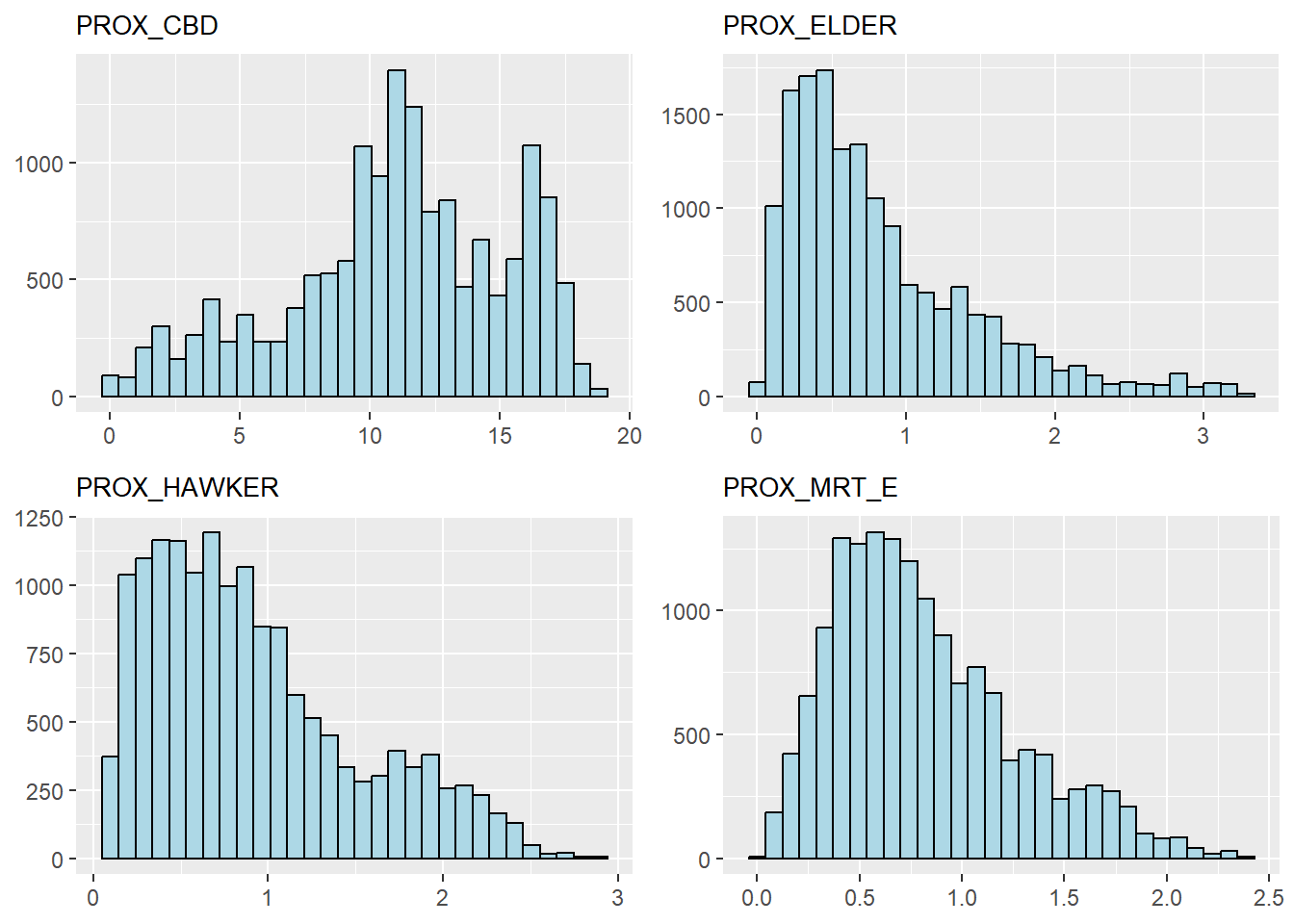
$`2`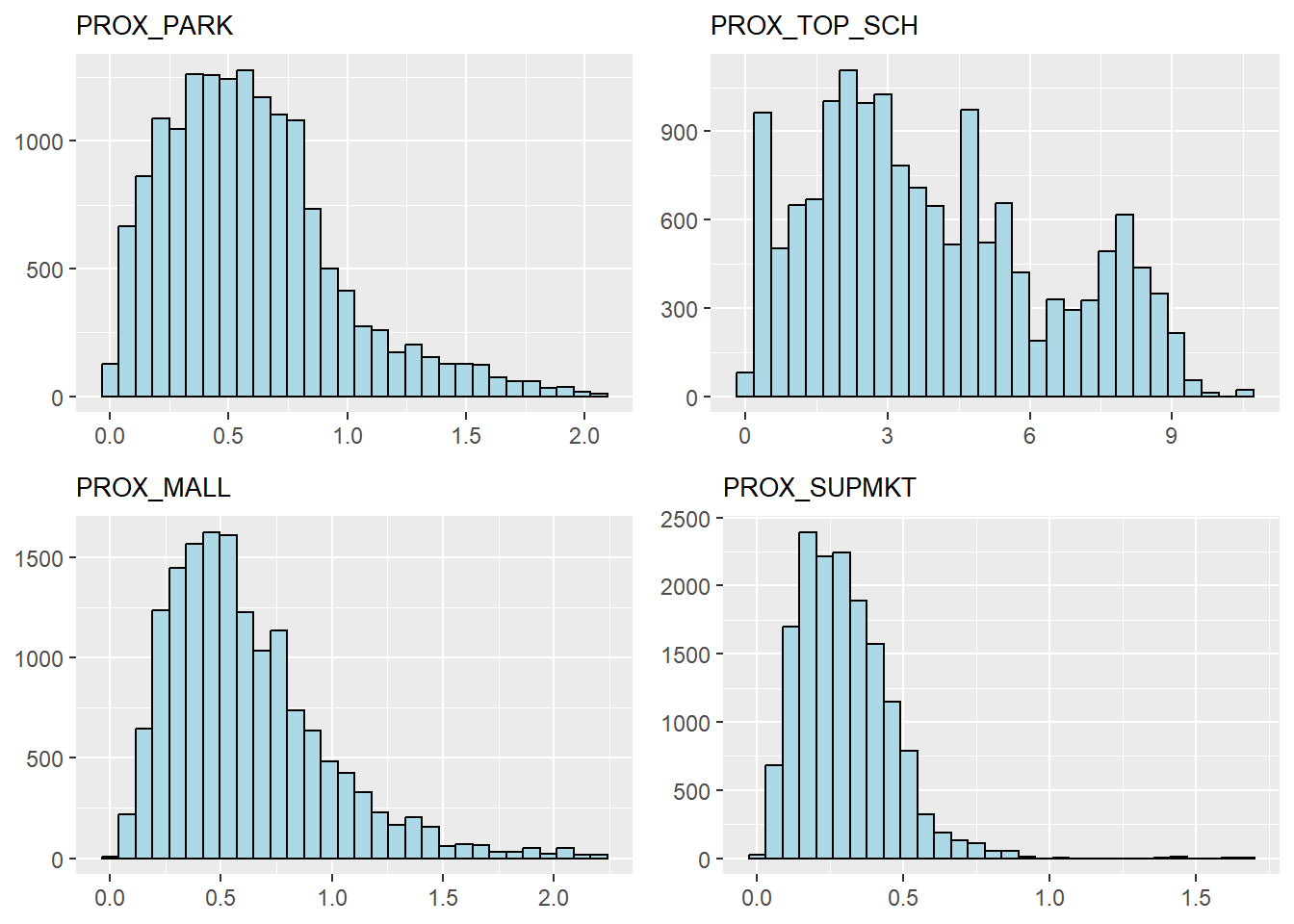
$`3`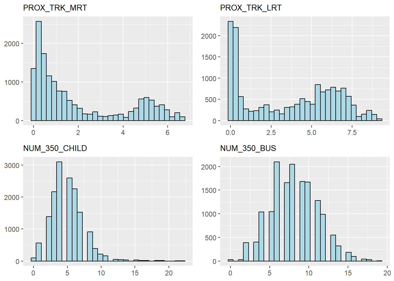
$`4`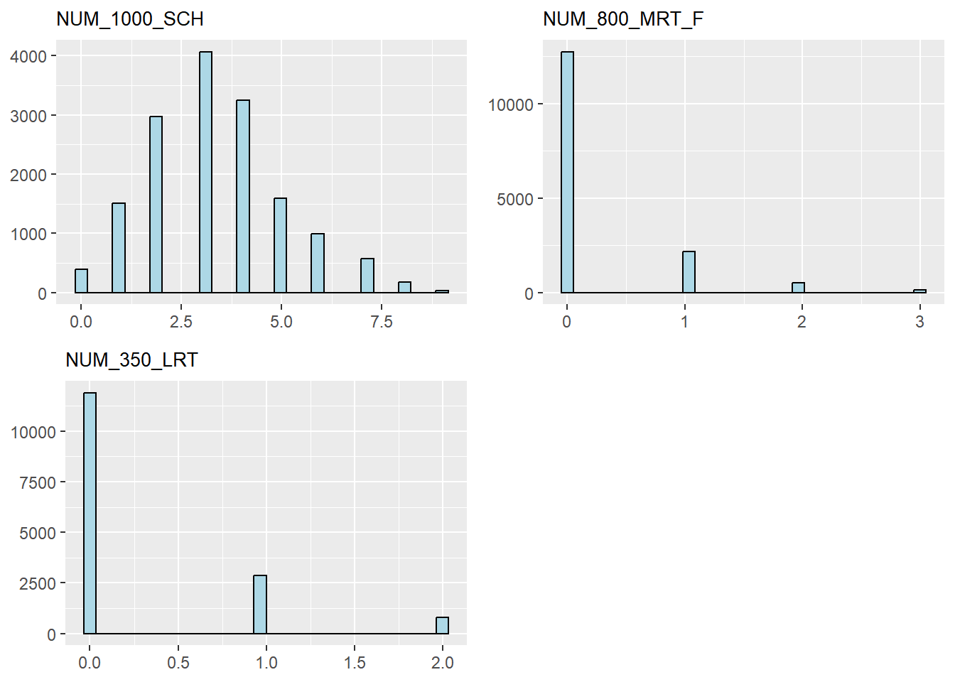
attr(,"class")
[1] "list" "ggarrange"Proximity:
Proximity to CBD is somewhat slightly left skewed, there are most houses that are about 11km away from the CBD
Proximity to Eldercare is very right skewed, most houses have an eldercare within 1km of their house
Proximity to Hawker centre is very right skewed, most houses have a hawker centre within 1km of their house
Proximity to the nearest existing MRT station is somewhat right skewed, with most houses having access to an MRT station within 1km. We can note the interesting trend that the peak is about 0.4km to 0.8km, meaning that the placement of MRT stations could be to obtain an optimum 0.4km to 0.8km to any housing.
Proximity to Parks is right skewed. Most people have access to a park in under 0.8km.
Proximity to good schools is somewhat slightly right skewed with multiple peaks. The highest peak being at about 2.5km and second highest peaks at 0.5km and 5km.
Proximity to malls is right skewed, peaking at 0.5km.
Proximity to supermarket is right skewed with a short tail, most houses can access a supermarket within 0.5km and at most 1 to 1.5km (outlier).
Proximity to elevated MRT track is somewhat right skewed.
The proximity to LRT track is also somewhat right skewed.
Number:
The number of childcare centres in 350m of a household is somewhat right skewed, Most houses have about 4.
The number of bus stops within 350m of a home i somewhat normally distributed, with most having about 6 bus stops.
The number of houses having a school within 1km of their homes is somewhat normally distributed, most having 3 schools
The number of future MRT stops within 800m of a home is extremely right skewed, with most homes having none.
The number of LRT stations within 350m of a home is extremely right skewed, with most homes having none.
7.5 Statistical Point Map
Let us explore more about the 5-room HDB resale dataset with its parameters.
With the code chunk below, we will generate external HTML Interactive Map pages which are appended with the proximity and within locational factors details in the popup bar in separate interactive maps.
Code
tmap_options("view")
statpt_tmap1 <- tm_shape(mpsz) +
tm_polygons("REGION_N",
alpha = 0.2) +
tm_shape(final_resale) +
tm_dots("resale_price",
popup.vars= c("month" = "month", "town" = "town", "block" = "block", "street_name" = "street_name", "floor_area_sqm" = "floor_area_sqm", "resale_price" = "resale_price", "remaining_lease_mths" = "remaining_lease_mths", "PROX_CBD" = "PROX_CBD", "PROX_ELDER" = "PROX_ELDER", "PROX_HAWKER" = "PROX_HAWKER", "PROX_MRT_E" = "PROX_MRT_E", "PROX_PARK" = "PROX_PARK", "PROX_TOP_SCH" = "PROX_TOP_SCH", "PROX_MALL" = "PROX_MALL", "PROX_SUPMKT" = "PROX_SUPMKT", "PROX_TRK_MRT" = "PROX_TRK_MRT", "PROX_TRK_LRT" = "PROX_TRK_LRT", "NUM_350_CHILD"),
size = 0.05,
style = "quantile")
statpt_tmap2 <- tm_shape(mpsz) +
tm_polygons("REGION_N",
alpha = 0.2) +
tm_shape(final_resale) +
tm_dots("resale_price",
popup.vars= c("month" = "month", "town" = "town", "block" = "block", "street_name" = "street_name", "floor_area_sqm" = "floor_area_sqm", "resale_price" = "resale_price", "remaining_lease_mths" = "remaining_lease_mths", "NUM_350_CHILD" = "NUM_350_CHILD", "NUM_350_KINDER" = "NUM_350_KINDER", "NUM_350_BUS" = "NUM_350_BUS", "NUM_1000_SCH" = "NUM_1000_SCH", "NUM_800_MRT_F" = "NUM_800_MRT_F", "NUM_350_LRT" = "NUM_350_LRT", "storey_order" = "storey_order", "multistorey" = "multistorey", "model_standard" = "model_standard", "model_dbss" = "model_dbss", "model_adjoined" = "model_adjoined", "model_3gen" = "model_3gen", "model_s2" = "model_s2", "hip" = "hip", "mup" = "mup"),
size = 0.05,
style = "quantile")
tmap_save(statpt_tmap1, "thex03_statpt_tmap1.html")
tmap_save(statpt_tmap2, "thex03_statpt_tmap2.html")View Interactive Version of Map with Proximity Locational Factors Here! [39+mb]
View Interactive Version of Map with Within Locational Factors Here! [44+mb]
Using the code chunk below, we will generate the interactive map of resale prices using quantile style. The difference compared to the above maps are that the popup variables are not generated.
Code
tmap_options("view")named list()Code
tm_shape(mpsz) +
tm_polygons("REGION_N",
alpha = 0.2) +
tm_shape(final_resale) +
tm_dots("resale_price",
size = 0.05,
style = "quantile")7.6 Computing Correlation Matrix
Before we create the OLS and Machine Learning Models to predict housing prices, we need to check if there is any strong correlation which suggests multicollinearity. We will drop one of the variable if there is a pair which correlation above 0.8 (very strong positive correlation) or below -0.8 (very strong negative correlation).
The code chunk below exports the correlation plot into a png so that the text is more readable and image is higher in resolution.
final_resale_nogeom <- final_resale %>% st_drop_geometry()
png(file="Take-Home_Ex03/corr.png", res=300, width=2500, height=2000)
corrplot::corrplot(cor(final_resale_nogeom[,c(5, 7:34)]),
diag = FALSE,
order = "AOE",
tl.pos = "td",
tl.cex = 0.5,
number.cex = 0.4,
number.font = 2,
number.digits = 2,
method = "number",
type = "upper")
while (!is.null(dev.list())) dev.off()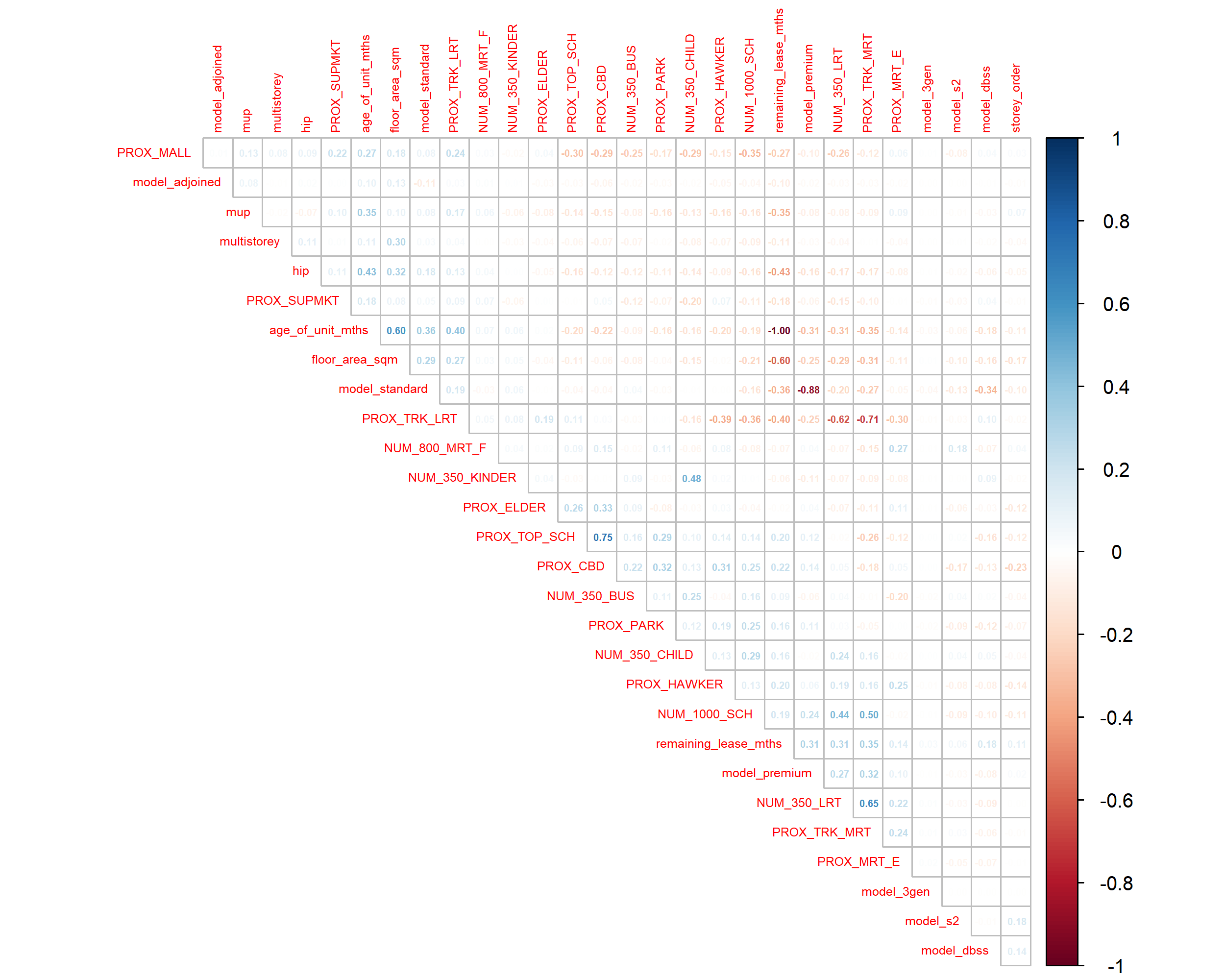
From the correlation matrix above, we can see that:
age_of_unit_mthsandremaining_lease_mthshave perfect negative correlation since theage_of_unit_mthswas derived using(99 years x 12 mths) - remaining_lease_mths. In this case, we will removeage_of_unit_mthsmodel_standardandmodel_premiumhas a very strong negative correlation of -0.88 since in most scenerios, if a unit is not a standard one, it is premium. We will remove themodel_premiumvariable
Using the code chunk below, we will drop the two variables selected, age_of_unit_mths and model_premium.
final_resale <- select(final_resale, c(-age_of_unit_mths, -model_premium))7.7 Preparing Model and Test Data
For our models, we want to use data from Jan 2021 to Dec 2022 to build our model and Jan to Feb 2023 to predict and test our models. The code below will help us split the dataset into two:
resale.model <- final_resale %>% filter(!month %in% c("2023-01", "2023-02"))
resale.test <- final_resale %>% filter(month %in% c("2023-01", "2023-02"))8 OLS Multiple Linear Regression Model
8.1 Building the OLS Model using olsrr
Code
resale.mlr <- lm(formula = resale_price ~ floor_area_sqm + remaining_lease_mths + PROX_CBD + PROX_ELDER + PROX_HAWKER + PROX_MRT_E + PROX_PARK + PROX_TOP_SCH + PROX_MALL + PROX_SUPMKT + PROX_TRK_MRT + PROX_TRK_LRT + NUM_350_CHILD + NUM_350_BUS + NUM_1000_SCH + NUM_800_MRT_F + NUM_350_LRT + storey_order + multistorey + model_standard + model_dbss + model_adjoined + model_3gen + model_s2 + hip + mup,
data = resale.model)
ols_regress(resale.mlr) Model Summary
--------------------------------------------------------------------------
R 0.877 RMSE 70231.211
R-Squared 0.769 MSE 4941593019.242
Adj. R-Squared 0.769 Coef. Var 11.213
Pred R-Squared 0.768 AIC 366089.961
MAE 54090.948 SBC 366302.351
--------------------------------------------------------------------------
RMSE: Root Mean Square Error
MSE: Mean Square Error
MAE: Mean Absolute Error
AIC: Akaike Information Criteria
SBC: Schwarz Bayesian Criteria
ANOVA
--------------------------------------------------------------------------------
Sum of
Squares DF Mean Square F Sig.
--------------------------------------------------------------------------------
Regression 2.391957e+14 26 9.199834e+12 1861.714 0.0000
Residual 7.176676e+13 14523 4941593019.242
Total 3.109624e+14 14549
--------------------------------------------------------------------------------
Parameter Estimates
-----------------------------------------------------------------------------------------------------------------
model Beta Std. Error Std. Beta t Sig lower upper
-----------------------------------------------------------------------------------------------------------------
(Intercept) -200694.423 18255.977 -10.993 0.000 -236478.464 -164910.383
floor_area_sqm 5064.577 112.912 0.253 44.854 0.000 4843.256 5285.899
remaining_lease_mths 574.521 6.934 0.568 82.855 0.000 560.930 588.113
PROX_CBD -20356.350 260.469 -0.595 -78.153 0.000 -20866.903 -19845.797
PROX_ELDER -3082.035 1073.922 -0.013 -2.870 0.004 -5187.058 -977.012
PROX_HAWKER -13074.269 1229.070 -0.053 -10.638 0.000 -15483.402 -10665.136
PROX_MRT_E -61341.007 1614.105 -0.187 -38.003 0.000 -64504.859 -58177.155
PROX_PARK -14932.379 1862.872 -0.037 -8.016 0.000 -18583.845 -11280.914
PROX_TOP_SCH -1112.042 399.198 -0.019 -2.786 0.005 -1894.520 -329.563
PROX_MALL -34678.564 1993.365 -0.085 -17.397 0.000 -38585.813 -30771.315
PROX_SUPMKT -39774.014 3984.014 -0.043 -9.983 0.000 -47583.189 -31964.839
PROX_TRK_MRT -11756.273 553.079 -0.164 -21.256 0.000 -12840.377 -10672.168
PROX_TRK_LRT 5414.990 359.107 0.106 15.079 0.000 4711.095 6118.885
NUM_350_CHILD -1490.883 277.269 -0.024 -5.377 0.000 -2034.366 -947.401
NUM_350_BUS -862.774 215.761 -0.018 -3.999 0.000 -1285.694 -439.854
NUM_1000_SCH -4454.142 501.272 -0.051 -8.886 0.000 -5436.699 -3471.586
NUM_800_MRT_F 18989.313 1211.401 0.071 15.675 0.000 16614.812 21363.814
NUM_350_LRT 9174.366 1526.316 0.035 6.011 0.000 6182.592 12166.140
storey_order 18543.067 300.515 0.267 61.704 0.000 17954.019 19132.116
multistorey 77573.192 6625.359 0.050 11.709 0.000 64586.644 90559.739
model_standard -20719.741 1763.984 -0.057 -11.746 0.000 -24177.374 -17262.108
model_dbss 101665.105 4034.083 0.120 25.202 0.000 93757.788 109572.422
model_adjoined -7285.709 11064.846 -0.003 -0.658 0.510 -28974.216 14402.798
model_3gen 11548.544 31528.081 0.001 0.366 0.714 -50250.509 73347.597
model_s2 100298.838 9795.242 0.046 10.240 0.000 81098.916 119498.759
hip 31951.001 2168.971 0.070 14.731 0.000 27699.542 36202.460
mup 64250.029 3800.711 0.080 16.905 0.000 56800.152 71699.906
-----------------------------------------------------------------------------------------------------------------Based on the results above, we can see that the P-Value for all except model_adjoined and model_3gen are statistically significant, meaning that it’s P-value (Sig) is more than or equal to 0.05. Hence, we cannot statistically conclude that the predictor is significant in contributing towards the model and we can safely remove them.
Code
resale.mlr <- lm(formula = resale_price ~ floor_area_sqm + remaining_lease_mths + PROX_CBD + PROX_ELDER + PROX_HAWKER + PROX_MRT_E + PROX_PARK + PROX_TOP_SCH + PROX_MALL + PROX_SUPMKT + PROX_TRK_MRT + PROX_TRK_LRT + NUM_350_CHILD + NUM_350_BUS + NUM_1000_SCH + NUM_800_MRT_F + NUM_350_LRT + storey_order + multistorey + model_standard + model_dbss + model_s2 + hip + mup,
data = resale.model)
ols_regress(resale.mlr) Model Summary
--------------------------------------------------------------------------
R 0.877 RMSE 70232.595
R-Squared 0.769 MSE 4941107221.972
Adj. R-Squared 0.769 Coef. Var 11.212
Pred R-Squared 0.768 AIC 366086.534
MAE 54093.835 SBC 366283.753
--------------------------------------------------------------------------
RMSE: Root Mean Square Error
MSE: Mean Square Error
MAE: Mean Absolute Error
AIC: Akaike Information Criteria
SBC: Schwarz Bayesian Criteria
ANOVA
--------------------------------------------------------------------------------
Sum of
Squares DF Mean Square F Sig.
--------------------------------------------------------------------------------
Regression 2.391929e+14 24 9.966369e+12 2017.032 0.0000
Residual 7.176958e+13 14525 4941107221.972
Total 3.109624e+14 14549
--------------------------------------------------------------------------------
Parameter Estimates
-----------------------------------------------------------------------------------------------------------------
model Beta Std. Error Std. Beta t Sig lower upper
-----------------------------------------------------------------------------------------------------------------
(Intercept) -200360.698 18231.074 -10.990 0.000 -236095.924 -164625.471
floor_area_sqm 5057.331 112.101 0.253 45.114 0.000 4837.599 5277.063
remaining_lease_mths 574.757 6.926 0.568 82.980 0.000 561.180 588.333
PROX_CBD -20346.293 260.077 -0.595 -78.232 0.000 -20856.077 -19836.510
PROX_ELDER -3079.302 1073.718 -0.013 -2.868 0.004 -5183.925 -974.679
PROX_HAWKER -13062.464 1228.235 -0.053 -10.635 0.000 -15469.961 -10654.967
PROX_MRT_E -61340.649 1613.927 -0.187 -38.007 0.000 -64504.151 -58177.146
PROX_PARK -14937.606 1862.156 -0.037 -8.022 0.000 -18587.669 -11287.543
PROX_TOP_SCH -1120.702 398.956 -0.019 -2.809 0.005 -1902.707 -338.698
PROX_MALL -34631.820 1992.305 -0.085 -17.383 0.000 -38536.992 -30726.648
PROX_SUPMKT -39794.106 3983.639 -0.043 -9.989 0.000 -47602.545 -31985.667
PROX_TRK_MRT -11751.542 553.006 -0.164 -21.250 0.000 -12835.503 -10667.580
PROX_TRK_LRT 5419.382 359.023 0.106 15.095 0.000 4715.652 6123.112
NUM_350_CHILD -1494.085 277.139 -0.024 -5.391 0.000 -2037.313 -950.856
NUM_350_BUS -865.015 215.725 -0.018 -4.010 0.000 -1287.863 -442.166
NUM_1000_SCH -4446.884 501.066 -0.051 -8.875 0.000 -5429.037 -3464.731
NUM_800_MRT_F 18978.819 1211.259 0.071 15.669 0.000 16604.597 21353.041
NUM_350_LRT 9179.434 1526.223 0.035 6.014 0.000 6187.842 12171.026
storey_order 18545.941 300.440 0.267 61.729 0.000 17957.039 19134.842
multistorey 77774.669 6615.547 0.050 11.756 0.000 64807.354 90741.983
model_standard -20542.854 1736.679 -0.057 -11.829 0.000 -23946.965 -17138.743
model_dbss 101757.629 4028.813 0.120 25.257 0.000 93860.644 109654.615
model_s2 100519.587 9788.110 0.046 10.270 0.000 81333.646 119705.528
hip 31983.397 2168.387 0.070 14.750 0.000 27733.081 36233.712
mup 64167.356 3798.164 0.080 16.894 0.000 56722.472 71612.240
-----------------------------------------------------------------------------------------------------------------After removing the model_adjoined and model_3Gen columns, the rest of the P-values are < 0.05, which means all variables statistically explain the OLS Multiple Linear Regression model. Also note that the Adj. R-Squred value did not change and RMSE had only a minor change in value.
8.2 Testing for Linear Regression Assumptions
ols_vif_tol(resale.mlr) Variables Tolerance VIF
1 floor_area_sqm 0.5054852 1.978297
2 remaining_lease_mths 0.3392932 2.947303
3 PROX_CBD 0.2746794 3.640608
4 PROX_ELDER 0.7261788 1.377071
5 PROX_HAWKER 0.6459490 1.548110
6 PROX_MRT_E 0.6585302 1.518533
7 PROX_PARK 0.7499854 1.333359
8 PROX_TOP_SCH 0.3515751 2.844342
9 PROX_MALL 0.6710724 1.490152
10 PROX_SUPMKT 0.8502706 1.176096
11 PROX_TRK_MRT 0.2657027 3.763605
12 PROX_TRK_LRT 0.3245823 3.080883
13 NUM_350_CHILD 0.7849905 1.273901
14 NUM_350_BUS 0.7837533 1.275912
15 NUM_1000_SCH 0.4822043 2.073810
16 NUM_800_MRT_F 0.7815098 1.279575
17 NUM_350_LRT 0.4731388 2.113545
18 storey_order 0.8494672 1.177208
19 multistorey 0.8762886 1.141177
20 model_standard 0.6843937 1.461147
21 model_dbss 0.7072066 1.414014
22 model_s2 0.7969990 1.254707
23 hip 0.7057126 1.417007
24 mup 0.7121516 1.404195From the code chunk above, we can see that there is no high Multicolinearity between the variables (VIF above 5). Hence, the Multicolinearity assumption is valid.
ols_plot_resid_fit(resale.mlr)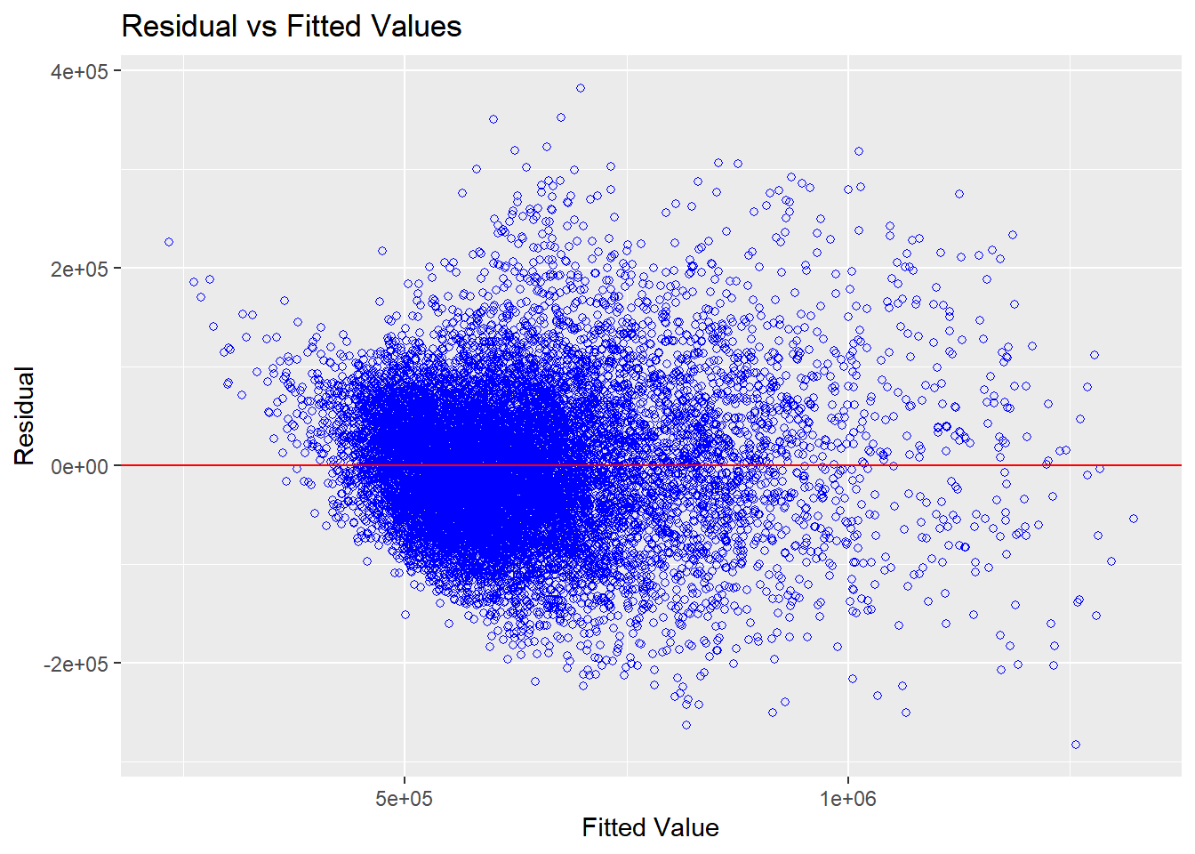
Next, by viewing the plot above, we can see that most values are somewhat clustered along the 0 line and are somewhat linear. Hence, we can say that the Non-Linearity assumption is valid.
ols_plot_resid_hist(resale.mlr)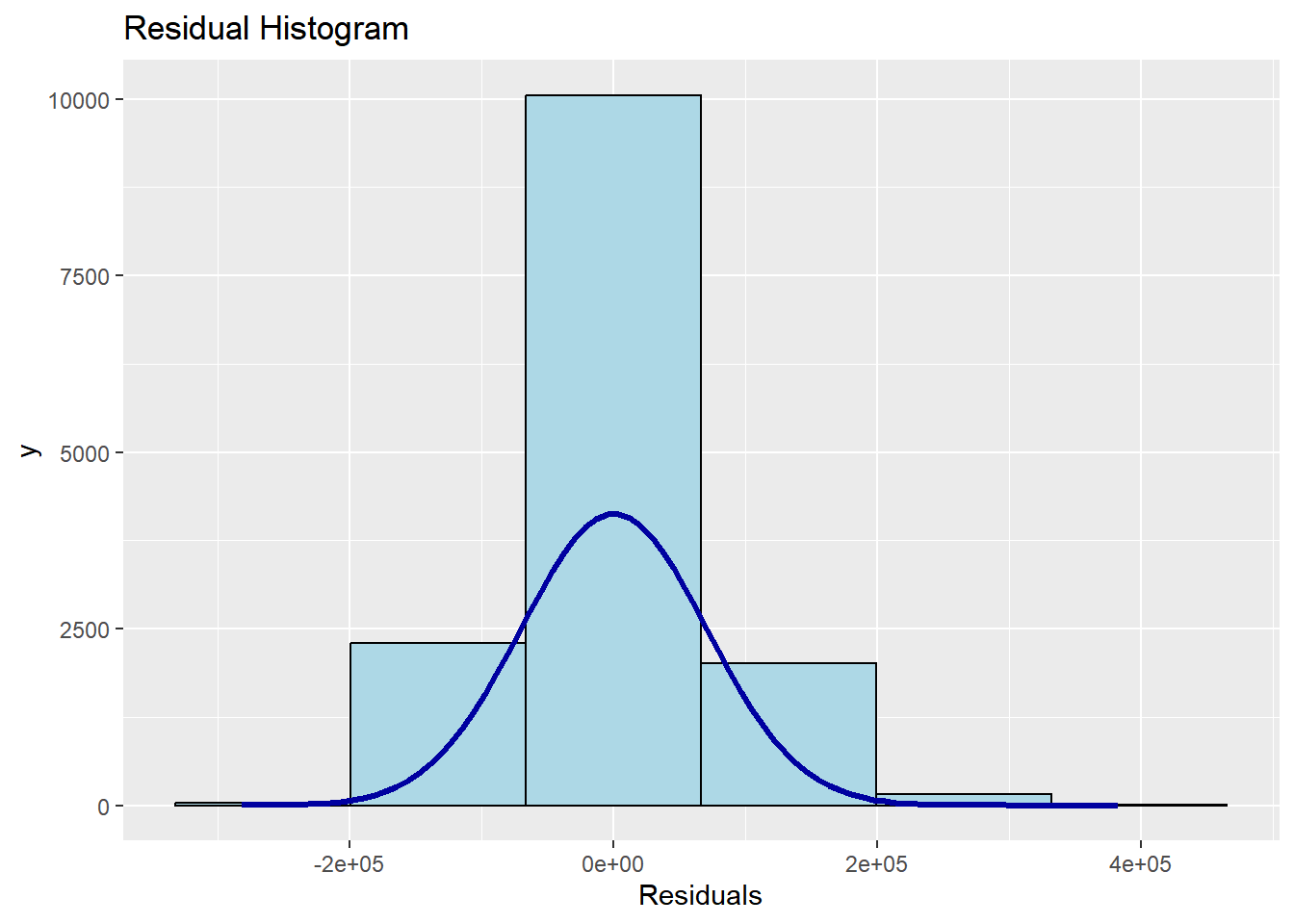
The graph above plots the residuals, we can see that the residuals are normallly distributed hence, the normality assumption is valid.
Firstly, we will convert the residual plots to Spatial Points Data Frame for further analysis later.
resale.mlr.residuals <- as.data.frame(resale.mlr$residuals)
final_resale.mlr.residuals <- cbind(resale.model, resale.mlr.residuals) %>%
rename(`MLR_RES` = `resale.mlr.residuals`)
final_resale.mlr.sp <- as_Spatial(final_resale.mlr.residuals)
final_resale.mlr.spclass : SpatialPointsDataFrame
features : 14550
extent : 11519.79, 42645.18, 28157.26, 48741.06 (xmin, xmax, ymin, ymax)
crs : +proj=tmerc +lat_0=1.36666666666667 +lon_0=103.833333333333 +k=1 +x_0=28001.642 +y_0=38744.572 +ellps=WGS84 +towgs84=0,0,0,0,0,0,0 +units=m +no_defs
variables : 33
names : month, town, block, street_name, floor_area_sqm, resale_price, remaining_lease_mths, PROX_CBD, PROX_ELDER, PROX_HAWKER, PROX_MRT_E, PROX_PARK, PROX_TOP_SCH, PROX_MALL, PROX_SUPMKT, ...
min values : 2021-01, ANG MO KIO, 1, ADMIRALTY DR, 99, 350000, 589, 0.0661807920161801, 3.24787909339429e-07, 0.0494878683160973, 0.0117455829446405, 0.00670893634680754, 0.104811675233461, 0, 7.48064072230297e-07, ...
max values : 2022-12, YISHUN, 9B, ZION RD, 167, 1418000, 1161, 18.8605387305912, 3.28231365739252, 2.84445163777424, 2.39772594334572, 2.0666519572555, 10.6431215873685, 2.20277079513291, 1.67131003232231, ... Next, we plot a tmap to see the residual plots of resale units.
tmap_mode("view")
tm_shape(mpsz) +
tm_polygons("REGION_N",
alpha = 0.5) +
tm_shape(final_resale.mlr.sp) +
tm_dots("MLR_RES",
size = 0.05)From our plot above, we can see that there are signs of spatial autocorrelation. To confirm our observation is statistically true, we can perofrm the Moran’s I Test. Using the code chunk below, we will calculate in sequence:
- Obtain the distance-based weight matrixusing dnearneigh() using spdep
- Convert neighbour lists (nb) into spatial weights
- Perofrm the Moran’s I Test
nb <- dnearneigh(coordinates(final_resale.mlr.sp), 0, 1500, longlat = FALSE)
nb_lw <- nb2listw(nb, style = 'W')
lm.morantest(resale.mlr, nb_lw)
Global Moran I for regression residuals
data:
model: lm(formula = resale_price ~ floor_area_sqm +
remaining_lease_mths + PROX_CBD + PROX_ELDER + PROX_HAWKER + PROX_MRT_E
+ PROX_PARK + PROX_TOP_SCH + PROX_MALL + PROX_SUPMKT + PROX_TRK_MRT +
PROX_TRK_LRT + NUM_350_CHILD + NUM_350_BUS + NUM_1000_SCH +
NUM_800_MRT_F + NUM_350_LRT + storey_order + multistorey +
model_standard + model_dbss + model_s2 + hip + mup, data =
resale.model)
weights: nb_lw
Moran I statistic standard deviate = 427.54, p-value < 2.2e-16
alternative hypothesis: greater
sample estimates:
Observed Moran I Expectation Variance
2.120058e-01 -6.768898e-04 2.474684e-07 From the results in the code chunk above:
- Since the P-value is < 0.05, we will reject the null hypothesis that the spatial points are randomly distributed.
- Since the Observed Moran I value is > 0, we can conclude that the spatial points resemble cluster distribution
From here, since the points resemble cluster distribution, it might be a good idea to explore Geographically Weighted methods that takes into account the neighbouring points and clustering effect which may obtain a better result.
8.3 Predicting OLS Multiple Linear Regression Model
Using the code chunk below, we will first seperate out the test Dataframe to one that is specifically for Multiple Linear Regression before we merge the predicted results into the Data Frame.
resale.mlrtest <- resale.test
resale.mlrtest$predict <- predict(object = resale.mlr, newdata = resale.mlrtest)Next, we calculate the error in prediction for all rows using the formula predict - resale_price. A negative value means a precition that is below the actual resale price.
resale.mlrtest <- resale.mlrtest %>% mutate(error = resale.mlrtest$predict - resale.mlrtest$resale_price)8.3.1 Calculating RMSE
Using the rmse() function, we can obtain the rmse score of the test data for Jan and Feb 2023 resale data for future comparison later.
rmse(resale.mlrtest$resale_price,
resale.mlrtest$predict)[1] 84198.88.4 Visualising Interactive Mpa of Errors
Next, we can plot a interactive tmap of errors using quantile style to explore the errors.
Code
tmap_mode("view")
tm_shape(mpsz) +
tm_polygons("REGION_N",
alpha = 0.2) +
tm_shape(resale.mlrtest) +
tm_dots("error",
size = 0.05,
style = "quantile")8.5 Visualising the Predicted Values
Using the code below, we can plot a scatterplot of the predicted values.
mlr.plot <- ggplot(data = resale.mlrtest,
aes(x = predict,
y = resale_price)) +
geom_point()
ggplotly(mlr.plot)As you can see, the predicted values are mostly scattered along an imaginary line, which is good as this shows that the model is a good predictive model. We can also mouse over to see the outlier points that do not confirm close to the imaginary line.
9 Geographical Random Forest Model
9.1 Preparing Data
To obtain the bandwidth using bw.gwr() method, we need to pass the data in as a Spatial Points Data Frame. First, we will conver the resale training data (resale.model) as resale.rf.sp
resale.rf.sp <- as_Spatial(resale.model)Next, the Geographical Random Forest Model building and predictive method requires data to be formatted in a certain way. Building the model requires coordinate data and model data to be seperated.
resale.rf.coords <- st_coordinates(resale.model)
resale.rf <- resale.model %>% st_drop_geometry()Laslt,y test data requires geometry information not as a sf DataFrame but tibble Data Frame with X Y columns. The code chunk below will format it into the necessary format.
resale.rftest.coords <- st_coordinates(resale.test)
resale.rftest <- cbind(resale.test,resale.rftest.coords) %>% st_drop_geometry()9.2 Locating Optimum Bandwidth Selection
Next, we need to obtain the optimum bandwidth to be used for building our Geographically Weighted Random Forest model. Using the code chunk below, we can obtain it.
The code takes very long to run, hence it is not evaluated but the end result is a value that can be used in the bw parameter when building the model.
bw_adaptive <- bw.gwr(formula = resale_price ~ floor_area_sqm + remaining_lease_mths + PROX_CBD + PROX_ELDER + PROX_HAWKER + PROX_MRT_E + PROX_PARK + PROX_TOP_SCH + PROX_MALL + PROX_SUPMKT + PROX_TRK_MRT + PROX_TRK_LRT + NUM_350_CHILD + NUM_350_BUS + NUM_1000_SCH + NUM_800_MRT_F + NUM_350_LRT + storey_order + multistorey + model_standard + model_dbss + model_adjoined + model_3gen + model_s2 + hip + mup,
data = resale.rf.sp,
approach="CV",
kernel="gaussian",
adaptive=TRUE,
longlat=FALSE)Similarly as above, we save the bandwidth to an rds file so that we do not need to run the code everytime on render. The data will be loaded using read_rds from the respective directory.
write_rds(bw_adaptive, "Take-Home_Ex03/model/bw_adaptive.rds")bw_adaptive <- read_rds("Take-Home_Ex03/model/bw_adaptive.rds")9.3 Building Random Forest Model
Utilising grf() of SpatialML, we can build a Geographically Weighted Random Forest model by inputting the paramter to be predicted, its predictors, dataframe (without coordinates), bandwidth, type of kernel and coordinates as a seperate dataframe.
set.seed(1234)
gwRF_adaptive <- grf(formula = resale_price ~ floor_area_sqm + remaining_lease_mths + PROX_CBD + PROX_ELDER + PROX_HAWKER + PROX_MRT_E + PROX_PARK + PROX_TOP_SCH + PROX_MALL + PROX_SUPMKT + PROX_TRK_MRT + PROX_TRK_LRT + NUM_350_CHILD + NUM_350_BUS + NUM_1000_SCH + NUM_800_MRT_F + NUM_350_LRT + storey_order + multistorey + model_standard + model_dbss + model_adjoined + model_3gen + model_s2 + hip + mup,
dframe = resale.rf,
bw = bw_adaptive,
kernel = "adaptive",
coords = resale.rf.coords)Similarly, since the model takes 2 hours to run and model size is about 50GB, we will save it as and RDS file to prevent rerunning it everytime on render. We also save the results into another seperate file called gwRF_results so prevent loading the entire 50GB model when we just need to view the results and importance of variables.
write_rds(gwRF_adaptive, "Take-Home_Ex03/model/gwRF_adaptive.rds")
gwRF_results <- gwRF_adaptive[["Global.Model"]]
write_rds(gwRF_results, "Take-Home_Ex03/model/gwRF_results.rds")
gwRF_adaptive <- read_rds("Take-Home_Ex03/model/gwRF_adaptive.rds")This code chunk below shows the results from the building of the GWRF model.
gwRF_results <- read_rds("Take-Home_Ex03/model/gwRF_results.rds")
gwRF_resultsRanger result
Call:
ranger(resale_price ~ floor_area_sqm + remaining_lease_mths + PROX_CBD + PROX_ELDER + PROX_HAWKER + PROX_MRT_E + PROX_PARK + PROX_TOP_SCH + PROX_MALL + PROX_SUPMKT + PROX_TRK_MRT + PROX_TRK_LRT + NUM_350_CHILD + NUM_350_BUS + NUM_1000_SCH + NUM_800_MRT_F + NUM_350_LRT + storey_order + multistorey + model_standard + model_dbss + model_adjoined + model_3gen + model_s2 + hip + mup, data = resale.rf, num.trees = 500, mtry = 8, importance = "impurity", num.threads = NULL)
Type: Regression
Number of trees: 500
Sample size: 14550
Number of independent variables: 26
Mtry: 8
Target node size: 5
Variable importance mode: impurity
Splitrule: variance
OOB prediction error (MSE): 1644508284
R squared (OOB): 0.9230584 We can also understand the importance of each parameter to the Geographically Weighted Random Forest Model.
gwRF_results[["variable.importance"]] floor_area_sqm remaining_lease_mths PROX_CBD
1.390021e+13 5.443985e+13 8.323953e+13
PROX_ELDER PROX_HAWKER PROX_MRT_E
7.997121e+12 9.368938e+12 1.558666e+13
PROX_PARK PROX_TOP_SCH PROX_MALL
5.089762e+12 2.503078e+13 7.197148e+12
PROX_SUPMKT PROX_TRK_MRT PROX_TRK_LRT
3.439543e+12 9.554883e+12 1.059239e+13
NUM_350_CHILD NUM_350_BUS NUM_1000_SCH
1.954534e+12 2.095376e+12 4.191898e+12
NUM_800_MRT_F NUM_350_LRT storey_order
6.806918e+11 8.623046e+11 3.564587e+13
multistorey model_standard model_dbss
7.944169e+11 5.537918e+12 7.522683e+12
model_adjoined model_3gen model_s2
9.897470e+10 1.710756e+09 6.113985e+11
hip mup
3.203755e+11 3.419251e+11 From the above code, we can see which predictors are most important towards contributing to the final predicted resale results. The top five most important parameters are:
- Proximity to LRT Track (
PROX_TRK_LRT) - Floor Area in SQM (
floor_area_sqm) - Proximity to Elevated MRT Track (
PROX_MRT_E) - Proximity to Top School (
PROX_TOP_SCH) - Which storey is it (
storey_order)
9.4 Predicting Test Data
We can use the predict.grf() function to predict our test dataset of 5-room HDB resale units between Jan to Feb 2023 as prepared earlier.
gwRF_pred <- predict.grf(gwRF_adaptive,
resale.rftest,
x.var.name="X",
y.var.name="Y",
local.w=1,
global.w=0)Similarly as above, we save the predicted results as RDS to prevent rerunning the predictive model. The few code chunks below will also reload the dataset and combine the predicted results into the test dataset resale.rftest using cbind(). We will also save the data as RDS to prevent having to reload and reprocess the data.
GRF_pred <- write_rds(gwRF_pred, "Take-Home_Ex03/model/GRF_pred.rds")GRF_pred <- read_rds("Take-Home_Ex03/model/GRF_pred.rds")
GRF_pred_df <- as.data.frame(GRF_pred)test_data_p <- cbind(resale.rftest, GRF_pred_df)write_rds(test_data_p, "Take-Home_Ex03/model/test_data_p.rds")test_data_p <- read_rds("Take-Home_Ex03/model/test_data_p.rds")9.4.1 Caculating RMSE
The code chunk below calculates the error using the predicted value - the actual resale pricing and merges it to another column with geometry so that we can plot it on a tmap later.
test_data_p <- mutate(test_data_p, error = GRF_pred - resale_price)
resale.rftest.tmap <- cbind(resale.test, test_data_p$error)
names(resale.rftest.tmap)[names(resale.rftest.tmap) == 'test_data_p.error'] <- "error"Using the rmse() function, we can find out what the rmse score for the model so that we can compare it later.
rmse(test_data_p$resale_price,
test_data_p$GRF_pred)[1] 55008.959.5 Visualising the Predicted Values
Using the code below, we can plot a scatterplot of the predicted values.
gwrf.plot <- ggplot(data = test_data_p,
aes(x = GRF_pred,
y = resale_price)) +
geom_point()
ggplotly(gwrf.plot)As you can see, thepredicted values are mostly scattered along an imaginary line, which is good as this shows that the model is a good predictive model. We can also mouseover to see the outlier points that do not confirm close to the imaginary line.
9.6 Visualisation of Errors
Using the interactive tmap beloow, we can plot a map of errors to explore how the Geographically Weighted Random Forest model has improved the prediction of housing prices.
Code
tmap_mode("view")
tm_shape(mpsz) +
tm_polygons("REGION_N",
alpha = 0.1) +
tm_shape(resale.rftest.tmap) +
tm_dots("error",
size = 0.05,
alpha = 0.7,
style = "quantile")We will go further into the comparative analysis of OLS Multiple Linear Regression Model and Geographically Weighted Random Forest models in the next section below.
10 Comparative Analysis
Now that we have completed building and predicting the the OLS Linear Regression and SpatialML’s Geographically Weighted Random Forest model performance, let us do a side-by-side comparison of both model’s performance.
10.1 Parameters for Each Model
As a recap, we will include predictors used in each model. Both models predict the HDB resale prices between Jan and Feb 2023 and are trained on HDB resale data between Jan 2021 to Dec 2022.
OLS Multiple Linear Regression does not contain model_3Gen and model_adjoined parameters as based on analysis by the model, the two parameters are not statistically significant to the model and are removed.
| OLS Multiple Linear Regression | Geographically Weighted Random Forest |
|---|---|
| Floor Area SQM | Floor Area SQM |
| Remaining Lease (Months) | Remaining Lease (Months) |
| Proximity to CBD (Downtown Core Boundary - Linestring) in km | Proximity to CBD (Downtown Core Boundary - Linestring) in km |
| Proximity to Eldercare in km | Proximity to Eldercare in km |
| Proximity to Hawker Centre in km | Proximity to Hawker Centre in km |
| Proximity to Existing MRT Station in km | Proximity to Existing MRT Station in km |
| Proximity to Park (Boundary - Linestring) in km | Proximity to Park (Boundary - Linestring) in km |
| Proximity to Good Primary School in km | Proximity to Good Primary School in km |
| Proximity to Mall in km | Proximity to Mall in km |
| Proximity to Supermarket in km | Proximity to Supermarket in km |
| Proximity to MRT Overground Track in km | Proximity to MRT Overground Track in km |
| Proximity to LRT Overground Track in km | Proximity to LRT Overground Track in km |
| Number of Childcare in 350m Radius | Number of Childcare in 350m Radius |
| Number of Bus Stops in 350m Radius | Number of Bus Stops in 350m Radius |
| Number of Primary Schools in 1km | Number of Primary Schools in 1km |
| Number of Future MRT stations in 800m | Number of Future MRT stations in 800m |
| Number of LRT stations in 350m | Number of LRT stations in 350m |
| HDB Storey Level - Recoded Values (+1 = +3 stories) | HDB Storey Level - Recoded Values (+1 = +3 stories) |
| Multistorey Apartment (1 - True, 0 - False) | Multistorey Apartment (1 - True, 0 - False) |
| Standard Type Apartment (1 - True, 0 - False) | Standard Type Apartment (1 - True, 0 - False) |
| DBSS Type Apartment (1 - True, 0 - False) | DBSS Type Apartment (1 - True, 0 - False) |
| S2 Type Apartment (1 - True, 0 - False) | Adjoined Type Apartment (1 - True, 0 - False) |
| Home Improvement Programme (1 - True, 0 - False) | 3Gen Type Apartment (1 - True, 0 - False) |
| Main Upgrading Programme (1 - True, 0 - False) | S2 Type Apartment (1 - True, 0 - False) |
| Home Improvement Programme (1 - True, 0 - False) | |
| Main Upgrading Programme (1 - True, 0 - False) |
10.2 General Statistics
10.2.1 Root Mean Squared Error (RMSE)
To compare across different models, we typically use the RMSE value generated from predicting the test values using the trained data to find out how does the model perform on data it has never seen before.
The RMSE value can be derived by sqrt((y actual - y predicted)^2).
| OLS Multiple Linear Regression | Geographically Weighted Random Forest | |
|---|---|---|
| RMSE | 84198.8 | 55089.5 |
The OLS Multiple Linear Regression has a RMSE error of 84198.8, meaning, the mean error for the HDB resale prices prediction is +/- $84198.80. Similarly for Geographically Weighted Random Forest, the mean error for HDB resale prices prediction is +/- $55089.50.
As we can see, OLS Multiple Linear Regression has a higher RMSE score than Geographically Weighted Random Forest. Hence, the Geographically Weighted Random Forest is a better model as there are lesser deviations in error
10.2.2 Box Plot
Now, we will plot a boxplot to see the distribution of errors and its outliers.
Code
boxplot <- plot_ly(x = resale.mlrtest$error, type = "box", name = "OLS MLR")
boxplot <- boxplot %>% add_trace(x = resale.rftest.tmap$error, name = "GWRF")
boxplot The boxplot is interactive, you may tap the plot to inspect the points and statistics of each boxplot.
From our box plot, we can see that the GWRF model is better in OLS MLR model in all aspects:
- GWR has a less most extreme (negative and positive) outlier as compared to OLS MLR model
- GWR a smaller range of error between the 0th Quartile and 4th Quartile, meaning that the range of errors is lesser than OLS MLR model
- GWR’s range of errors are closer to zero, meaning predictions are closer to actual resale price of HDBs than OLS MLR model
10.2.3 Understanding RMSE by Town
To understand the RMSE improvements at town levels from the OLS MLR model to the GWRF model, we can calculate the RMSE scores at HDB town level by filter and calculating the RMSE scores using each model’s predicted resale price and the actual resale price.
The code chunk below extracts unique HDB towns, loops through the town names to create a dataframe containing the HDB town name, OLS RMSE score, GWRF RMSE score and the change in RMSE score from OLS to GWR. A positive score means an improvement from OLS to GWRF (ie. the errors reduced from OLS to GWRF).
TOWN <- unique(resale.mlrtest$town)
RMSE_TOWN <- data.frame()
for (t in TOWN){
x <- filter(resale.mlrtest, resale.mlrtest$town == t)
y <- filter(test_data_p, test_data_p$town == t)
xr <- rmse(x$resale_price, x$predict)
yr <- rmse(y$resale_price, y$GRF_pred)
row <- data.frame(town = t, olsrmse = xr, gwrfrmse = yr)
RMSE_TOWN <- rbind(RMSE_TOWN, row)
}
RMSE_TOWN <- RMSE_TOWN %>% mutate(change_rmse = RMSE_TOWN$olsrmse - RMSE_TOWN$gwrfrmse)
RMSE_TOWN[order(-RMSE_TOWN$change_rmse),] town olsrmse gwrfrmse change_rmse
18 QUEENSTOWN 204643.53 52788.48 151855.055
15 MARINE PARADE 193284.34 84276.77 109007.570
3 BISHAN 164108.13 69224.13 94884.000
17 PUNGGOL 102508.66 41495.72 61012.946
9 CLEMENTI 151823.14 94805.04 57018.100
5 BUKIT MERAH 116460.98 67249.40 49211.573
4 BUKIT BATOK 103740.26 58454.36 45285.902
21 SERANGOON 104325.20 62940.52 41384.679
6 BUKIT PANJANG 75396.71 35020.34 40376.366
16 PASIR RIS 85079.90 49637.31 35442.595
12 JURONG EAST 70699.10 39511.79 31187.308
7 CENTRAL AREA 159241.41 130937.23 28304.185
25 YISHUN 68596.49 41816.71 26779.775
1 ANG MO KIO 106734.75 80537.22 26197.531
10 GEYLANG 79480.26 54568.51 24911.743
8 CHOA CHU KANG 63943.20 40352.40 23590.798
24 WOODLANDS 64160.62 42264.54 21896.081
13 JURONG WEST 63789.10 44813.36 18975.742
20 SENGKANG 57409.74 40902.13 16507.605
23 TOA PAYOH 106676.87 92966.82 13710.044
19 SEMBAWANG 45841.68 38336.30 7505.384
22 TAMPINES 63875.32 59416.10 4459.228
14 KALLANG/WHAMPOA 85529.29 83465.06 2064.235
11 HOUGANG 74549.95 82154.33 -7604.377
2 BEDOK 63599.00 80728.54 -17129.537From viewing the changes of RMSE in different HDB towns, we can see that the RMSE scores improved in all towns except Bedok and Hougang .
This means that for predictions of HDB resale prices in all towns except Bedok and Hougang, they became more accurate moving from OLS Multiple Linear Regression model to Geographically Weighted Random Forest model. Only Bedok’s and Hougang’s resale pricing predictions became worse, Bedok by -$17129.53 in mean root mean squared errors and Hougang by -$7604.37 in RMSE.
More investigation would have to be done to understand further about why the two towns, Bedok and Hougang, became worse at predicting HDB resale prices with the GWRF model.
10.3 Map Comparison
10.3.1 Plot of Errors
Code
tmap_mode("view")
t1 <- tm_shape(mpsz) +
tm_polygons("REGION_N",
alpha = 0.1) +
tm_shape(resale.mlrtest) +
tm_dots("error",
size = 0.05,
alpha = 0.7,
breaks = c(-Inf, -200000, -100000, -75000, -50000, -25000, 0, 25000, 50000, 75000, Inf))
t2 <- tm_shape(mpsz) +
tm_polygons("REGION_N",
alpha = 0.1) +
tm_shape(resale.rftest.tmap) +
tm_dots("error",
size = 0.05,
alpha = 0.7,
breaks = c(-Inf, -200000, -100000, -75000, -50000, -25000, 0, 25000, 50000, 75000, Inf))
tmap_arrange(t1, t2, ncol = 2, sync = TRUE)10.4 Comparative Analysis of RMSE by Towns
Let us zoom into the specific HDB towns and compare the predicted errors between OLS Multiple Linear Regression and Geographically Weighted Random Forest models.
For reference, the interactive map on the left is the results from OLS Multiple Linear Regression Model and the right is from the Geographically Weighted Random Forest.
We have chosen a list of towns from different regions of Singapore that was designed with different planning principles and built in different time periods:
- Jurong West - West
- Woodlands - North
- Punggol - North East
- Tampines - East
- Bukit Merah - Central
10.4.1 Generate Error by Town Function
Using the function below, we can plot interactive tmaps of errors in different HDB towns by calling the generate_error_town with 2 spatial dataframes and the HDB Town (AREA) to be filtered. A side-byside tmap will be generated and movement will be synced across both maps.
generate_error_town <- function(geo1, geo2, AREA) {
tmap_mode("view")
plot_map_t1 <- filter(geo1, town == AREA)
plot_map_t2 <- filter(geo2, town == AREA)
t1 <-
tm_shape(plot_map_t1) +
tm_dots("error",
size = 0.05,
alpha = 0.7,
breaks = c(-Inf, -200000, -100000, -75000, -50000, -25000, 0, 25000, 50000, 75000, Inf)) +
tm_view(set.zoom.limits = c(14, 16))
t2 <-
tm_shape(plot_map_t2) +
tm_dots("error",
size = 0.05,
alpha = 0.7,
breaks = c(-Inf, -200000, -100000, -75000, -50000, -25000, 0, 25000, 50000, 75000, Inf)) +
tm_view(set.zoom.limits = c(14, 16))
tmap_arrange(t1, t2, ncol = 2, sync = TRUE)
}10.4.2 Generate RMSE by Town
The code block below will generate the RMSE (Root Mean Squared Errors) for each HDB Town specified. This measure could be used to compare:
- Same model, across towns
- Different model, same dataset (town or full dataset)
This could give us a sensing of how well the model is good at predicting each area’s reasale house pricings.
Sample Code for Yishun:
RMSE_TOWN %>% filter(town == "YISHUN") town olsrmse gwrfrmse change_rmse
1 YISHUN 68596.49 41816.71 26779.7710.4.3 Jurong West - West
Code
generate_error_town(resale.mlrtest, resale.rftest.tmap, "JURONG WEST")(left): OLS Multiple Linear Regression | (right): Geographically Weighted Random Forest
Code
RMSE_TOWN %>% filter(town == "JURONG WEST") town olsrmse gwrfrmse change_rmse
1 JURONG WEST 63789.1 44813.36 18975.74There are lesser extreme errors in the Geographically Weighted Random Forest model from the OLS Multiple Linear Regression model, the Root Mean Squared Error (RMSE) for Jurong West fell from $63789.10 to $44813.36 when moving from OLS to GWRF models.. Most predicted HDB resale pricing is closer to 0.
Takeaway points:
- Best improved cluster of HDB resale units were near Corporation Rd and Corporation Dr to the South West corner of Jurong Lake Gardens. The predicted values in the GWRF model was close to actual pricing (within +/- 25,000).
- GWRF could have improved the model as it learns and weighs points differently based on its Geographical locations and neighbours. It acknowledges clustering effects and adjusts the weights based on its parameter values, hence, better generalising and predicting resale pricing values.
10.4.4 Woodlands - North
Code
generate_error_town(resale.mlrtest, resale.rftest.tmap, "WOODLANDS")(left): OLS Multiple Linear Regression | (right): Geographically Weighted Random Forest
Code
RMSE_TOWN %>% filter(town == "WOODLANDS") town olsrmse gwrfrmse change_rmse
1 WOODLANDS 64160.62 42264.54 21896.08There are lesser extreme errors in the Geographically Weighted Random Forest model from the OLS Multiple Linear Regression model, the Root Mean Squared Error (RMSE) for Woodlands fell from $64160.62 to $42264.54 when moving from OLS to GWRF models.. Most predicted HDB resale pricing is closer to 0.
Takeaway points:
- Most HDB predictions improved from -$200,000 to -$75,000 errors from Predicted to Actual resale values to $-50,000 to $0 error, going from OLS MLR model to GWRF model. This means that the GWRF model can more accurately in most instances, predict housing prices closer to its actual values.
- GWRF could have improved the model as it learns and weighs points differently based on its Geographical locations and neighbours. It acknowledges clustering effects and adjusts the weights based on its parameter values, hence, better generalising and predicting resale pricing values. However, the GWRF model may have worsened the predictions for certain specific HDBs, specifically the ones right beside the MRT station (Admiralty and Woodlands MRT stations).
10.4.5 Punggol - North East
Code
generate_error_town(resale.mlrtest, resale.rftest.tmap, "PUNGGOL")(left): OLS Multiple Linear Regression | (right): Geographically Weighted Random Forest
Code
RMSE_TOWN %>% filter(town == "PUNGGOL") town olsrmse gwrfrmse change_rmse
1 PUNGGOL 102508.7 41495.72 61012.95There are lesser extreme errors in the Geographically Weighted Random Forest model from the OLS Multiple Linear Regression model, the Root Mean Squared Error (RMSE) for Punggol fell from $102508.70 to $41495.72 when moving from OLS to GWRF models.. Most predicted HDB resale pricing is closer to 0.
Takeaway points:
Most HDB predictions improved from -$200,000 to -$100,000 errors from Predicted to Actual resale values to $-25,000 to $0 error, going from OLS MLR model to GWRF model. This means that the GWRF model can more accurately in most instances, predict housing prices closer to its actual values.
GWRF has improved the model as it learns and weighs points differently based on its Geographical locations and neighbours. It acknowledges clustering effects and adjusts the weights based on its parameter values, hence, better generalising and predicting resale pricing values.
As we see, most resale housing in Punggol were closer to the actual predicted values, meaning that there is a general possibility of increased popularity of Punggol HDB resale units that could not be captured or interpreted using a Linear Regression model without context of Geographic clustering or with the predictors.
We can also understand this from Statistical Point Map if we zoom into Punggol area where the apartment units in Waterway Eastand Matilda estates are mostly in the very high outlier region. Hence, normal Linear Regression models cannot generalise this effect which may not be very well explained by the variables in put and be better understood by understanding the effects of clustering.
In this scenerio, we can see the importance of Geographic Weighted methods if clustering is observed between points as there might be unknown correlation that cannot be seen or interpreted without the knowledge of geospatial data.
10.4.6 Tampines - East
Code
generate_error_town(resale.mlrtest, resale.rftest.tmap, "TAMPINES")(left): OLS Multiple Linear Regression | (right): Geographically Weighted Random Forest
Code
RMSE_TOWN %>% filter(town == "TAMPINES") town olsrmse gwrfrmse change_rmse
1 TAMPINES 63875.32 59416.1 4459.228There are lesser extreme errors
There are lesser extreme errors in the Geographically Weighted Random Forest model from the OLS Multiple Linear Regression model, the Root Mean Squared Error (RMSE) for Tampines fell from $63875.32 to $59416.10 when moving from OLS to GWRF models. Most predicted HDB resale pricing is closer to 0.
Takeaway points:
- Most HDB predictions improved from -$75,000 to -$50,000 errors from Predicted to Actual resale values to $-50,000 to $0 error, going from OLS MLR model to GWRF model. This means that the GWRF model can more accurately in most instances, predict housing prices closer to its actual values.
- However, we also observe more instances of over-prediction of HDB resale pricing near the edges of Tampines
- GWRF could have improved the model as it learns and weighs points differently based on its Geographical locations and neighbours. It acknowledges clustering effects and adjusts the weights based on its parameter values, hence, better generalising and predicting resale pricing values.
10.4.7 Bukit Merah - Central
Code
generate_error_town(resale.mlrtest, resale.rftest.tmap, "BUKIT MERAH")(left): OLS Multiple Linear Regression | (right): Geographically Weighted Random Forest
Code
RMSE_TOWN %>% filter(town == "BUKIT MERAH") town olsrmse gwrfrmse change_rmse
1 BUKIT MERAH 116461 67249.4 49211.57There are lesser extreme errors in the Geographically Weighted Random Forest model from the OLS Multiple Linear Regression model, the Root Mean Squared Error (RMSE) for Bukit Merah fell from $116461 to $67249.40 when moving from OLS to GWRF models. Most predicted HDB resale pricing is closer to 0.
Takeaway points:
- Most HDB predictions improved from the extreme less than $-200,000 errors errors from Predicted to Actual resale values to $-25,000 to $0 error, going from OLS MLR model to GWRF model. This means that the GWRF model can more accurately in most instances, predict housing prices closer to its actual values.
- There are a few more instances of overprediction in the GWRF model though, between $25,000 to $75,000 to its actual resale value.
- GWRF could have improved the model as it learns and weighs points differently based on its Geographical locations and neighbours. It acknowledges clustering effects and adjusts the weights based on its parameter values, hence, better generalising and predicting resale pricing values.
In this case, Bukit Merah which is nearer to the Central Business District could have its pricing corrected more since the linear regression predictors cannot estimate the effects of proximity to CBD well enough, or, there could be unknown geographical effects seen in Punggol town where resale housing in the town could be seen as more attractive to buyers.
10.4.8 Bedok - East
Code
generate_error_town(resale.mlrtest, resale.rftest.tmap, "BEDOK")left): OLS Multiple Linear Regression | (right): Geographically Weighted Random Forest
Code
RMSE_TOWN %>% filter(town == "BEDOK") town olsrmse gwrfrmse change_rmse
1 BEDOK 63599 80728.54 -17129.54The Root Mean Squared Error (RMSE) for Bedok rose from $63,599 to $80728.54 when moving from OLS to GWRF models. Predicted HDB prices that were initially close to $0 predicted worse moving from OLS to GWRF models.
Takeaway points:
- There are a more instances of underprediction or extreme underprediction of HDB resale prices moving from OLS to GWRF models
- GWRF could have worsened the model as it learns and weighs points differently based on its Geographical locations and neighbours. It acknowledges clustering effects and adjusts the weights based on its parameter values, hence, better generalising and predicting resale pricing values. We cannot conclusively tell and conclude what factors made the GWRF model predict worse than the OLS model.
11 Conclusion
We would like to conclude off with some insights and lessons learnt from this exercise.
There are some predictors that may have no worked according to how we intended it to be. For example, by including the proximity data about Elevated MRT track in SIngapore, we want to see the impacts of noise to HDB units located closer to the track. However, based on our OLS Multiple Linear Regression model, this may not be the case. For every 1km away from the Elevated MRT track, housing prices drop by $11756.273 (+/- $553.079) from Building the OLS Model using olsrr earlier.
Next, from our analysis in selected towns (Punggol - North East), we learnt that in Punggol, the 4th most improved town in terms of RMSE , we know that factoring geographical clustering effects is very important as predictor values may not be sufficient in understanding resale prices in the area, there might be other factors such as supply demand or preference for resale apartments in the area.
In the case of Punggol, the large amounts of outlier resale apartments in Punggol could not inform the Linear Regression model adequately. Geographically Weighted Random Forest model could understanding the effects of clustering and adjust the resale prices in the area.
Another reason for that failure could be the Parks data set. As seen from Transform Parks Dataset, the way Punggol Waterway’ Park’s extents was highlighted only included the park region near Punggol Town Centre. However, it could be possible the housing prices along the entire Punggol Waterway stretch and the proximity of those housing cause housing prices to be increased. We could explore in future to include datasets such as Water Bodies or PCN data to improve the prediction.
On the other hand, Geographically Weighted Random Forest model could make predictions worse as seen in Hougang and Bedok (Bedok - East) where the generated results and its RMSE scores are worse off than using Multiple Linear Regression models. However, the results are inexplicable as ultimately, Random Forest models are black boxes and we cannot backtrack to understand which part of the algorithm or variables contributed to this bad prediction.
Additionally, the drawback of GWRF over OLS MLR is that GWRF takes very long to run and generates a model that is very large in size, making quick predictions impossible. However, given a longer term use case for more accurate predictions, GWRF can be considered with proper trial and error, tuning and exploration.
To end off, accessibility metrics could also be explored instead of distance to regions. Proximity distances may not be the most accurate measure, especially distances to faraway places such as the CBD or town centre as the same 5 kiloemtres can mean 10 minutes by train if its near a train station vs 30 minutes by bus or even 60mins if more walking is required. Accessibility metrics using network could be utilised to better measure buyer’s willingness to buy a flat based on time taken or convenience to certain key Points of Interests and locations.
12 Credits
Prof Kam Tin Seong - Lesson Materials
Nor Aisyah - Take Home Exercise 3
Megan Sim - Take Home Exercise 3
https://www.teoalida.com/singapore/hdbflattypes/
Relevant documentations of R Libraries