pacman::p_load(funModeling, sf, tidyverse, tmap, maptools, spatstat, raster)1 Overview
1.1 Setting the Scene
Water is an important resource to mankind. Clean and accessible water is critical to human health. It provides a healthy environment, a sustainable economy, reduces poverty and ensures peace and security. Yet over 40% of the global population does not have access to sufficient clean water. By 2025, 1.8 billion people will be living in countries or regions with absolute water scarcity, according to UN-Water. The lack of water poses a major threat to several sectors, including food security. Agriculture uses about 70% of the world’s accessible freshwater.
Developing countries are most affected by water shortages and poor water quality. Up to 80% of illnesses in the developing world are linked to inadequate water and sanitation. Despite technological advancement, providing clean water to the rural community is still a major development issues in many countries globally, especially countries in the Africa continent.
To address the issue of providing clean and sustainable water supply to the rural community, a global Water Point Data Exchange (WPdx) project has been initiated. The main aim of this initiative is to collect water point related data from rural areas at the water point or small water scheme level and share the data via WPdx Data Repository, a cloud-based data library. What is so special of this project is that data are collected based on WPDx Data Standard.
1.2 Objectives
Geospatial analytics hold tremendous potential to address complex problems facing society. In this study, you are tasked to apply appropriate spatial point patterns analysis methods to discover the geographical distribution of functional and non-function water points and their co-locations if any in Osun State, Nigeria.
1.3 Tasks
The specific tasks of this take-home exercise are as follows:
1.3.1 Exploratory Spatial Data Analysis (ESDA)
Derive kernel density maps of functional and non-functional water points. Using appropriate tmap functions,
Display the kernel density maps on openstreetmap of Osun State, Nigeria.
Describe the spatial patterns revealed by the kernel density maps. Highlight the advantage of kernel density map over point map.
1.3.2 Spatial Correlation Analysis
In this section, you are required to confirm statistically if the spatial distribution of functional and non-functional water points are independent from each other.
Formulate the null hypothesis and alternative hypothesis and select the confidence level.
Perform the test by using appropriate Second order spatial point patterns analysis technique.
With reference to the analysis results, draw statistical conclusions.
2 Getting Started
2.1 Data Acquisition
The following datasets would be used to study the geographical distribution of water points in Osun State in Nigeria.
| Dataset Name | Source |
|---|---|
| WPdx+ (wpdx_nga.csv) - Filtered by #clean_country_name from the website | WPdx Global Data Repositories |
| geoBoundaries Nigeria Level-1 Administrative Boundary (geoBoundaries-NGA-ADM1.shp) - UN OCHA CODs | geoBoundaries |
| Humanitarian Data Exchange Nigeria Level-1 Administrative Boundary (nga_admbnda_adm1_osgof_20190417.shp) | Humanitarian Data Exchange |
wpdx_nigeria.csv has been extracted to Take-Home_Ex01/data/aspatial. The two other geospatial datasets has been extracted to Take-Home_Ex01/data/geospatial.
2.2 Installing and Loading Packages
Next, pacman assists us by helping us load R packages that we require, sf, tidyverse and funModeling.
The following packages assists us to accomplish the following:
funModeling helps us with performing quick Data Exploration in R
sf helps to import, manage and process vector-based geospatial data in R
tidyverse which includes readr to import delimited text file, tidyr for tidying data and dplyr for wrangling data
tmap provides functions to allow us to plot high quality static or interactive maps using leaflet API
maptools provides us a set of tools for manipulating geographic data
spatstat has a wide range of functions for point pattern analysis
raster reads, writes, manipulates, analyses and model of gridded spatial data (raster)
3 Importing and Preparing Geospatial Data
3.1 Importing and Comparing Datasets
We have two geospatial shapefiles which indicates the the Nigeria Level-1 Administrative Boundary. However, we do not know which dataset is better suited for the task. Hence, we will do some data exploration to understand more about the attributes of each shapefile.
In the code below, dsn specifies the filepath where the dataset is located and layer provides the filename of the dataset excluding the file extension.
geoBoundaries_NGA = st_read(dsn = "Take-Home_Ex01/data/geospatial", layer = "geoBoundaries-NGA-ADM1")Reading layer `geoBoundaries-NGA-ADM1' from data source
`C:\renjie-teo\IS415-GAA\exercises\Take-Home_Ex01\data\geospatial'
using driver `ESRI Shapefile'
Simple feature collection with 37 features and 6 fields
Geometry type: MULTIPOLYGON
Dimension: XY
Bounding box: xmin: 2.668534 ymin: 4.273007 xmax: 14.67882 ymax: 13.89442
Geodetic CRS: WGS 84From the above message, it tells us that the dataset contains multipolygon features, containing 37 multipolygon features and 6 fields in the geoBoundaries_NGA simple feature data frame and is in the WGS84 geographic coordinates system.
Let us check the other dataset from Humanitarian data exchange.
HDX_NGA = st_read(dsn = "Take-Home_Ex01/data/geospatial", layer = "nga_admbnda_adm1_osgof_20190417")Reading layer `nga_admbnda_adm1_osgof_20190417' from data source
`C:\renjie-teo\IS415-GAA\exercises\Take-Home_Ex01\data\geospatial'
using driver `ESRI Shapefile'
Simple feature collection with 37 features and 12 fields
Geometry type: MULTIPOLYGON
Dimension: XY
Bounding box: xmin: 2.668534 ymin: 4.273007 xmax: 14.67882 ymax: 13.89442
Geodetic CRS: WGS 84From the above message, it tells us that the dataset contains multipolygon features, containing 37 multipolygon features and 12 fields in the HDX_NGA simple feature data frame and is in the WGS84 geographic coordinates system.
Let us compare the fields to determine which dataset would be sufficiently useful for our analysis.
head(geoBoundaries_NGA)Simple feature collection with 6 features and 6 fields
Geometry type: MULTIPOLYGON
Dimension: XY
Bounding box: xmin: 5.380235 ymin: 4.273007 xmax: 13.69222 ymax: 12.52145
Geodetic CRS: WGS 84
shapeName pcode level shapeID shapeGroup shapeType
1 Abia NG001 ADM1 NGA-ADM1-9716203B29245989 NGA ADM1
2 Adamawa NG002 ADM1 NGA-ADM1-9716203B34328871 NGA ADM1
3 Akwa Ibom NG003 ADM1 NGA-ADM1-9716203B9380274 NGA ADM1
4 Anambra NG004 ADM1 NGA-ADM1-9716203B31714231 NGA ADM1
5 Bauchi NG005 ADM1 NGA-ADM1-9716203B69582311 NGA ADM1
6 Bayelsa NG006 ADM1 NGA-ADM1-9716203B92894251 NGA ADM1
geometry
1 MULTIPOLYGON (((7.488712 4....
2 MULTIPOLYGON (((11.85399 7....
3 MULTIPOLYGON (((7.488712 4....
4 MULTIPOLYGON (((7.339063 6....
5 MULTIPOLYGON (((8.823522 10...
6 MULTIPOLYGON (((6.60183 4.3...head(HDX_NGA)Simple feature collection with 6 features and 12 fields
Geometry type: MULTIPOLYGON
Dimension: XY
Bounding box: xmin: 5.380235 ymin: 4.273007 xmax: 13.69222 ymax: 12.52145
Geodetic CRS: WGS 84
Shape_Leng Shape_Area ADM1_EN ADM1_PCODE ADM1_REF ADM1ALT1EN ADM1ALT2EN
1 4.695135 0.3965429 Abia NG001 Abia <NA> <NA>
2 11.525443 3.1130065 Adamawa NG002 Adamawa <NA> <NA>
3 5.263830 0.5494762 Akwa Ibom NG003 Akwa Ibom <NA> <NA>
4 3.595960 0.3926608 Anambra NG004 Anambra <NA> <NA>
5 13.952005 4.0110175 Bauchi NG005 Bauchi <NA> <NA>
6 5.046708 0.7767679 Bayelsa NG006 Bayelsa <NA> <NA>
ADM0_EN ADM0_PCODE date validOn validTo
1 Nigeria NG 2016-11-29 2019-04-17 <NA>
2 Nigeria NG 2016-11-29 2019-04-17 <NA>
3 Nigeria NG 2016-11-29 2019-04-17 <NA>
4 Nigeria NG 2016-11-29 2019-04-17 <NA>
5 Nigeria NG 2016-11-29 2019-04-17 <NA>
6 Nigeria NG 2016-11-29 2019-04-17 <NA>
geometry
1 MULTIPOLYGON (((7.38681 6.0...
2 MULTIPOLYGON (((13.62129 10...
3 MULTIPOLYGON (((8.344815 4....
4 MULTIPOLYGON (((6.932539 6....
5 MULTIPOLYGON (((10.75125 12...
6 MULTIPOLYGON (((6.552828 5....By comparing both datasets, the dataset from geoBoundaries is more favourable. Both tables contain similar values, such as name of state, state code and the deometry.
Humanitarian Data Exchange contains values such as its parent (ADM0). However, ADM0 is country level and since we are only looking at Osun State which is specifically in Nigeria, this data is not very relevant to our analysis.
The rest of the columns are not very relevant to the analysis to be conducted. Hence, we will pick geoBoundaries which has lesser irrelevant data to reduce size of data needed to compute the analysis.
The code below will remove the HDX_NGA dataset as we have determined that it is no longer required for our analysis.
remove(HDX_NGA)3.2 Coordinate Reference System
3.2.1 Checking the Coordinate Reference System
In the code below, we will check if the Coordinate Reference System has been specified correctly.
st_crs(geoBoundaries_NGA)Coordinate Reference System:
User input: WGS 84
wkt:
GEOGCRS["WGS 84",
ENSEMBLE["World Geodetic System 1984 ensemble",
MEMBER["World Geodetic System 1984 (Transit)"],
MEMBER["World Geodetic System 1984 (G730)"],
MEMBER["World Geodetic System 1984 (G873)"],
MEMBER["World Geodetic System 1984 (G1150)"],
MEMBER["World Geodetic System 1984 (G1674)"],
MEMBER["World Geodetic System 1984 (G1762)"],
MEMBER["World Geodetic System 1984 (G2139)"],
ELLIPSOID["WGS 84",6378137,298.257223563,
LENGTHUNIT["metre",1]],
ENSEMBLEACCURACY[2.0]],
PRIMEM["Greenwich",0,
ANGLEUNIT["degree",0.0174532925199433]],
CS[ellipsoidal,2],
AXIS["geodetic latitude (Lat)",north,
ORDER[1],
ANGLEUNIT["degree",0.0174532925199433]],
AXIS["geodetic longitude (Lon)",east,
ORDER[2],
ANGLEUNIT["degree",0.0174532925199433]],
USAGE[
SCOPE["Horizontal component of 3D system."],
AREA["World."],
BBOX[-90,-180,90,180]],
ID["EPSG",4326]]As seen above, the file has been configured correctly, having a WGS84 Geographic Coordinate System which maps to EPSG:4326.
3.2.2 Converting the Coordinate Reference System
What coordinate system do we utilise? Nigeria emcompasses 3 Universal Traverse Mercator (UTM) Zones, Zones 31N, 32N and 33N, each having its unique Projected Coordinate System. Let us refer to the figure below.
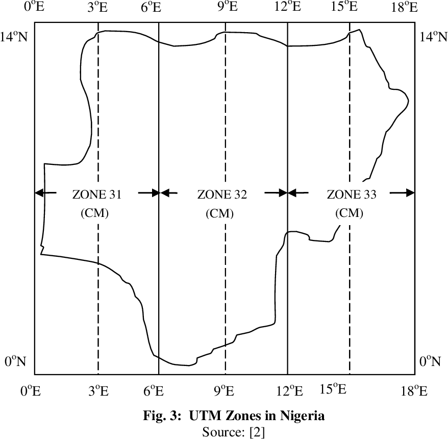
(Sylvester O et al., 2018)
Given that Osun State, Nigeria, has a coordinate of 7.5629° N, 4.5200° E which falls within Zone 31N, we would use the EPSG:26391 Projected Coordinate System which Zone 31N, Minna, Nigeria West Belt, corresponds to.
In the code below, we will convert the Geographic Coordinate Reference System from WGS84 to EPSG:26391 Projected Coordinate System:
nigeria <- st_transform(geoBoundaries_NGA, crs = 26391)st_crs(nigeria)Coordinate Reference System:
User input: EPSG:26391
wkt:
PROJCRS["Minna / Nigeria West Belt",
BASEGEOGCRS["Minna",
DATUM["Minna",
ELLIPSOID["Clarke 1880 (RGS)",6378249.145,293.465,
LENGTHUNIT["metre",1]]],
PRIMEM["Greenwich",0,
ANGLEUNIT["degree",0.0174532925199433]],
ID["EPSG",4263]],
CONVERSION["Nigeria West Belt",
METHOD["Transverse Mercator",
ID["EPSG",9807]],
PARAMETER["Latitude of natural origin",4,
ANGLEUNIT["degree",0.0174532925199433],
ID["EPSG",8801]],
PARAMETER["Longitude of natural origin",4.5,
ANGLEUNIT["degree",0.0174532925199433],
ID["EPSG",8802]],
PARAMETER["Scale factor at natural origin",0.99975,
SCALEUNIT["unity",1],
ID["EPSG",8805]],
PARAMETER["False easting",230738.26,
LENGTHUNIT["metre",1],
ID["EPSG",8806]],
PARAMETER["False northing",0,
LENGTHUNIT["metre",1],
ID["EPSG",8807]]],
CS[Cartesian,2],
AXIS["(E)",east,
ORDER[1],
LENGTHUNIT["metre",1]],
AXIS["(N)",north,
ORDER[2],
LENGTHUNIT["metre",1]],
USAGE[
SCOPE["Engineering survey, topographic mapping."],
AREA["Nigeria - onshore west of 6°30'E, onshore and offshore shelf."],
BBOX[3.57,2.69,13.9,6.5]],
ID["EPSG",26391]]After running the code, we can confirm that the data frame has been converted to EPSG:26391 Projected Coordinate System.
After converting to Projected Coordinated System, we no longer require the original dataset that was in the WGS84 Geographic Reference System. Let us remove it now.
remove(geoBoundaries_NGA)4 Importing and Preparing Aspatial Data
4.1 Importing WPdx+ Aspatial Data
Since WPdx+ data set is in csv format, we will use read_csv() of readr package to import wpdx_nigeria.csv and output it to an R object called wpdx.
wpdx <- read_csv("Take-Home_Ex01/data/aspatial/wpdx_nga.csv")list(wpdx)[[1]]
# A tibble: 97,478 × 74
row_id `#source` `#lat_deg` `#lon_deg` `#report_date` `#status_id`
<dbl> <chr> <dbl> <dbl> <chr> <chr>
1 158721 Federal Ministry of… 5.07 6.62 02/19/2015 12… Yes
2 158892 Federal Ministry of… 5.09 7.09 02/06/2015 12… Yes
3 323117 Federal Ministry of… 5.91 8.77 08/31/2015 12… Yes
4 300176 Federal Ministry of… 5.23 7.32 05/17/2015 12… Yes
5 324346 Federal Ministry of… 6.88 3.36 08/17/2015 12… Yes
6 297273 Federal Ministry of… 6.59 3.29 05/26/2015 12… Yes
7 296853 Federal Ministry of… 6.60 3.26 06/02/2015 12… Yes
8 323866 Federal Ministry of… 6.20 6.73 09/18/2015 12… Yes
9 297044 Federal Ministry of… 6.61 3.30 05/26/2015 12… Yes
10 324321 Federal Ministry of… 6.96 3.60 08/16/2015 12… Yes
# ℹ 97,468 more rows
# ℹ 68 more variables: `#water_source_clean` <chr>,
# `#water_source_category` <chr>, `#water_tech_clean` <chr>,
# `#water_tech_category` <chr>, `#facility_type` <chr>,
# `#clean_country_name` <chr>, `#clean_adm1` <chr>, `#clean_adm2` <chr>,
# `#clean_adm3` <lgl>, `#clean_adm4` <lgl>, `#install_year` <dbl>,
# `#installer` <lgl>, `#rehab_year` <lgl>, `#rehabilitator` <lgl>, …Our output shows our wpdx tibble data frame consists of 95,478 rows and 74 columns. The useful fields we would be paying attention to is the #lat_deg and #lon_deg columns, which are in the decimal degree format. By viewing the Data Standard on wpdx’s website, we know that the latitude and longitude is in the WGS84 Geographic Coordinate System.
Note
While wpdx contains all possible water points within nigeria at the moment, we still do not want to filter the data as some water points may be misclassified by state name (ie. a possible water point may be classified under an adjacent state name but physically is located in one state). We will filter the unrelated water points at a later stage.
4.1.1 Creating a Simple Feature Data Frame from an Aspatial Data Frame
As the geometry is available in wkt in the column New Georeferenced Column, we can use st_as_sfc() to import the geometry
wpdx$Geometry <- st_as_sfc(wpdx$`New Georeferenced Column`)As there is no spatial data information, firstly, we assign the original projection when converting the tibble dataframe to sf. The original is wgs84 which is EPSG:4326.
wpdx <- st_sf(wpdx, crs=4326)Next, we then convert the projection to the appropriate decimal based projection system. As discussed earlier, we utilise the EPSG:26391 Projected Coordinate System as Osun falls under Minna, Nigeria West Belt.
wpdx <- wpdx %>%
st_transform(crs = 26391)wpdxSimple feature collection with 97478 features and 74 fields
Geometry type: POINT
Dimension: XY
Bounding box: xmin: 32536.82 ymin: 33461.24 xmax: 1292096 ymax: 1091052
Projected CRS: Minna / Nigeria West Belt
# A tibble: 97,478 × 75
row_id `#source` `#lat_deg` `#lon_deg` `#report_date` `#status_id`
* <dbl> <chr> <dbl> <dbl> <chr> <chr>
1 158721 Federal Ministry of… 5.07 6.62 02/19/2015 12… Yes
2 158892 Federal Ministry of… 5.09 7.09 02/06/2015 12… Yes
3 323117 Federal Ministry of… 5.91 8.77 08/31/2015 12… Yes
4 300176 Federal Ministry of… 5.23 7.32 05/17/2015 12… Yes
5 324346 Federal Ministry of… 6.88 3.36 08/17/2015 12… Yes
6 297273 Federal Ministry of… 6.59 3.29 05/26/2015 12… Yes
7 296853 Federal Ministry of… 6.60 3.26 06/02/2015 12… Yes
8 323866 Federal Ministry of… 6.20 6.73 09/18/2015 12… Yes
9 297044 Federal Ministry of… 6.61 3.30 05/26/2015 12… Yes
10 324321 Federal Ministry of… 6.96 3.60 08/16/2015 12… Yes
# ℹ 97,468 more rows
# ℹ 69 more variables: `#water_source_clean` <chr>,
# `#water_source_category` <chr>, `#water_tech_clean` <chr>,
# `#water_tech_category` <chr>, `#facility_type` <chr>,
# `#clean_country_name` <chr>, `#clean_adm1` <chr>, `#clean_adm2` <chr>,
# `#clean_adm3` <lgl>, `#clean_adm4` <lgl>, `#install_year` <dbl>,
# `#installer` <lgl>, `#rehab_year` <lgl>, `#rehabilitator` <lgl>, …5 Geospatial Data Cleaning
5.1 Excluding Redundant Fields
As the nigeria sf dataframe consist of many redundant field, we use select() to select the fields which we want to retain. In our case, we will only retain the shapeName (State Name), pCode (State Code), shapeType (ADM Level) and geometry fields.
nigeria <- nigeria %>%
  dplyr::select(c(0:2, 6))
5.2 Checking for Duplicated State Names
It is important to check for duplicate name in the data main data fields. Using duplicated(), we can flag out state names that might be duplicated as shown below:
nigeria$ADM1_EN[duplicated(nigeria$ADM1_EN) == TRUE]NULLGreat! There are no duplicate state names.
Since our analysis is focused specifically on Osun state of Nigeria, we will extract the attributes related to Osun state into a new variable called nigeria_osun for further analysis.
nigeria_osun <- nigeria %>% filter(shapeName == "Osun")6 Data Wrangling for Water Point Data
6.1 Understanding Field Names
First, let us have a look at the #status_clean column which stores the information about Functional and Non-Functional data points. The code below returns all values that were used in the column.
funModeling::freq(data = wpdx,
     input = '#status_clean')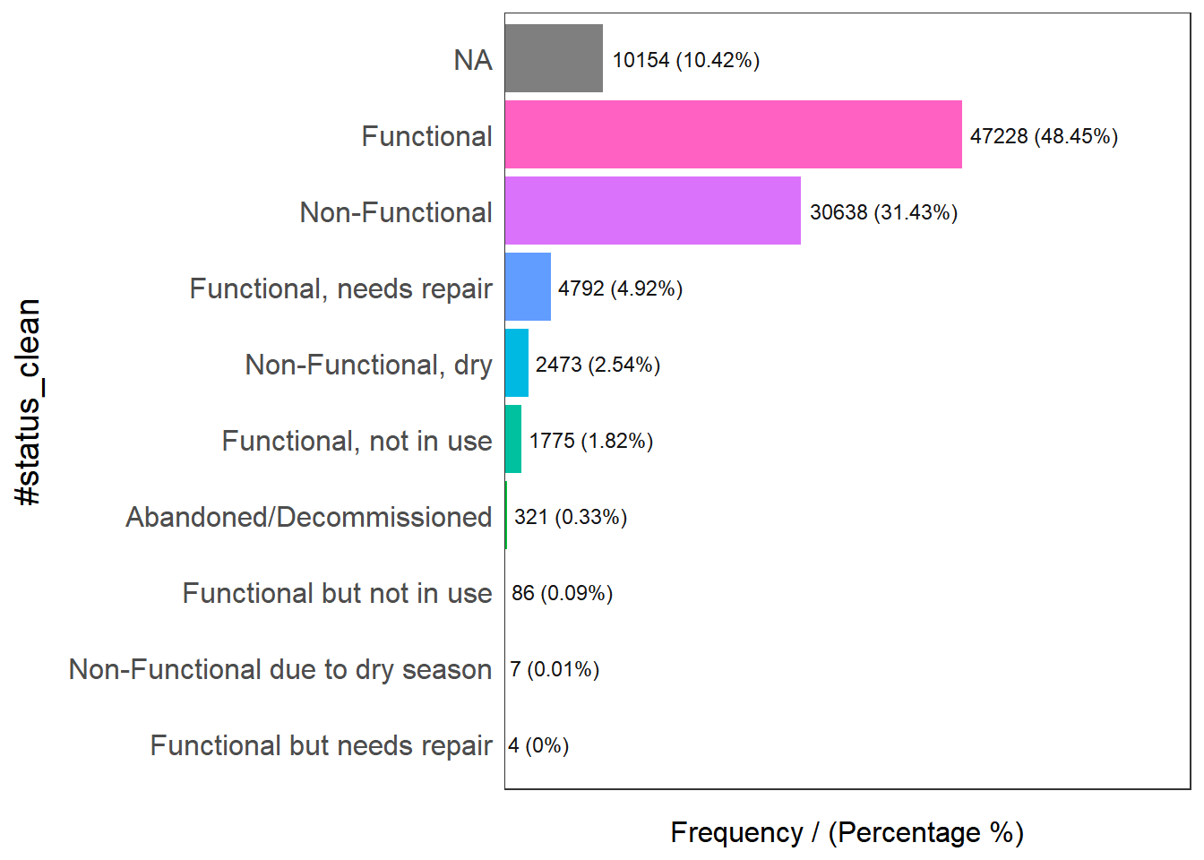
                      #status_clean frequency percentage cumulative_perc
1                        Functional     47228      48.45           48.45
2                    Non-Functional     30638      31.43           79.88
3                              <NA>     10154      10.42           90.30
4          Functional, needs repair      4792       4.92           95.22
5               Non-Functional, dry      2473       2.54           97.76
6            Functional, not in use      1775       1.82           99.58
7          Abandoned/Decommissioned       321       0.33           99.91
8         Functional but not in use        86       0.09          100.00
9  Non-Functional due to dry season         7       0.01          100.01
10      Functional but needs repair         4       0.00          100.00
As there might be issues performing mathematical calculations with NA labels, we will rename them to unknown.
The code below renames the column #status_clean to status_clean, select only the status_clean for manipulation and then replace all NA values to unknown.
wpdx <- wpdx %>%
  rename(status_clean = '#status_clean') %>%
  dplyr::select(status_clean) %>%
  mutate(status_clean = replace_na(status_clean, "unknown"))
6.2 Filtering Data
Firstly, since the wpdx dataset contains all data from all Nigeria states which is not required, let us use st_intersection() to filter out the unnecessary datapoints for our analysis. Using the code below, we keep points that are within nigeria_osun’s state boundary.
Note
Previously, we mentioned that some points may be misclassified as within a certain state but its coordinates may fall under another state. This method ensures that water points with its coordinates fall within the correct state boundary!
wpdx <- st_intersection(wpdx, nigeria_osun)With our previous knowledge, we can filter the data to obtain three main groups, Functional, Non-Functional and Unknown water points.
wpdx <- wpdx %>%
  mutate(status_clean = recode(status_clean,
                         `Functional but not in use` = 'Functional',
                         `Functional, not in use` = 'Functional',
                         `Functional, needs repair` =  'Functional',
                         `Abandoned/Decommissioned` = "Non-Functional",
                         `Non-Functional, dry` = "Non-Functional"))
wpdx_func <- wpdx %>%
filter(status_clean %in%
c("Functional",
"Functional but not in use",
"Functional, not in use",
"Functional, needs repair"))
wpdx_nonfunc <- wpdx %>%
filter(status_clean %in%
c("Abandoned/Decommissioned",
"Non-Functional",
"Non-Functional, dry"))
wpdx_unknown <- wpdx %>%
filter(status_clean == "unknown")
wpdx_excl_unknown <- wpdx %>%
filter(status_clean != "unknown")6.3 Plotting Map of Water Points
Using tmap, we can quickly plot a map of where the Functional, Non-Functional and Unknown water points are. We have plotted an interactive map which uses Openstreetmaps as its base layer so we can view each point’s location in relation to where roads, rivers, etc. are.
tmap_mode('view')
tm_basemap(server = "OpenStreetMap") +
tm_shape(nigeria_osun) +
  tm_polygons(alpha = 0.2) +
tm_shape(wpdx) +
  tm_dots("status_clean",
          alpha = 0.4,
          size = 0.05,
          palette = c("darkolivegreen2", "brown2", "cadetblue"))
With the help of Openstreetmaps base map, from a quick glance, it seems that water points are typically located near roads. There is more water points in certain areas, which could be attributed to being closer to urban centers or residential areas, given the denser layouts of roads.
In larger urban areas such as Osogobo in Osun, Nigeria, we can see clearly that there is a greater proportion of water points closer towards the centre of town.
However, it is hard for us to see the density of functional and non-functional water points from this map.
7 Geospatial Data Wrangling
7.1 Converting sf Dataframes to sp’s Spatial* Class
While simple feature data frame is gaining in popularity, many geospatial analysis packages still require the input geospatial data in sp’s Spatial* classes. We will convert the sf data frames to sp’s Spatial* Class below.
nigeria_osun_spat <- as_Spatial(nigeria_osun)
wpdx_spat <- as_Spatial(wpdx)
wpdx_func_spat <- as_Spatial(wpdx_func)
wpdx_nonfunc_spat <- as_Spatial(wpdx_nonfunc)
wpdx_excl_unknown_spat <- as_Spatial(wpdx_excl_unknown)
Now, let’s view the information of the Spatial* classes below:
nigeria_osun_spatclass : SpatialPolygonsDataFrame
features : 1
extent : 178398.7, 292278.9, 329463.4, 452734.9 (xmin, xmax, ymin, ymax)
crs : +proj=tmerc +lat_0=4 +lon_0=4.5 +k=0.99975 +x_0=230738.26 +y_0=0 +a=6378249.145 +rf=293.465 +towgs84=-92,-93,122,0,0,0,0 +units=m +no_defs
variables : 3
names : shapeName, pcode, shapeType
value : Osun, NG030, ADM1 wpdx_spatclass : SpatialPointsDataFrame
features : 5688
extent : 178980.8, 291989.5, 338261.8, 449013.7 (xmin, xmax, ymin, ymax)
crs : +proj=tmerc +lat_0=4 +lon_0=4.5 +k=0.99975 +x_0=230738.26 +y_0=0 +a=6378249.145 +rf=293.465 +towgs84=-92,-93,122,0,0,0,0 +units=m +no_defs
variables : 4
names : status_clean, shapeName, pcode, shapeType
min values : Functional, Osun, NG030, ADM1
max values : unknown, Osun, NG030, ADM1 wpdx_func_spatclass : SpatialPointsDataFrame
features : 2740
extent : 184202.3, 291989.5, 340352.2, 449013.7 (xmin, xmax, ymin, ymax)
crs : +proj=tmerc +lat_0=4 +lon_0=4.5 +k=0.99975 +x_0=230738.26 +y_0=0 +a=6378249.145 +rf=293.465 +towgs84=-92,-93,122,0,0,0,0 +units=m +no_defs
variables : 4
names : status_clean, shapeName, pcode, shapeType
min values : Functional, Osun, NG030, ADM1
max values : Functional, Osun, NG030, ADM1 wpdx_nonfunc_spatclass : SpatialPointsDataFrame
features : 2189
extent : 184218.5, 291855.5, 338261.8, 448933.5 (xmin, xmax, ymin, ymax)
crs : +proj=tmerc +lat_0=4 +lon_0=4.5 +k=0.99975 +x_0=230738.26 +y_0=0 +a=6378249.145 +rf=293.465 +towgs84=-92,-93,122,0,0,0,0 +units=m +no_defs
variables : 4
names : status_clean, shapeName, pcode, shapeType
min values : Non-Functional, Osun, NG030, ADM1
max values : Non-Functional, Osun, NG030, ADM1 wpdx_excl_unknown_spatclass : SpatialPointsDataFrame
features : 4929
extent : 184202.3, 291989.5, 338261.8, 449013.7 (xmin, xmax, ymin, ymax)
crs : +proj=tmerc +lat_0=4 +lon_0=4.5 +k=0.99975 +x_0=230738.26 +y_0=0 +a=6378249.145 +rf=293.465 +towgs84=-92,-93,122,0,0,0,0 +units=m +no_defs
variables : 4
names : status_clean, shapeName, pcode, shapeType
min values : Functional, Osun, NG030, ADM1
max values : Non-Functional, Osun, NG030, ADM1 Now, they have been correctly converted into sp’s Spatial* classes.
7.2 Converting the Spatial* Class into Generic sp Format
spstat requires the analytical data to be in ppp object form. As there is no direct method to convert Spatial* classes to ppp object, we need to convert the Spatial* classes into an intermediate Spatial object first.
The code below converts Spatial* Classes into generic sp objects
nigeria_osun_sp <- as(nigeria_osun_spat, "SpatialPolygons")
wpdx_sp <- as(wpdx_spat, "SpatialPoints")
wpdx_func_sp <- as(wpdx_func_spat, "SpatialPoints")
wpdx_nonfunc_sp <- as(wpdx_nonfunc_spat, "SpatialPoints")
Next, we can check the sp object properties.
nigeria_osun_spclass : SpatialPolygons
features : 1
extent : 178398.7, 292278.9, 329463.4, 452734.9 (xmin, xmax, ymin, ymax)
crs : +proj=tmerc +lat_0=4 +lon_0=4.5 +k=0.99975 +x_0=230738.26 +y_0=0 +a=6378249.145 +rf=293.465 +towgs84=-92,-93,122,0,0,0,0 +units=m +no_defs wpdx_spclass : SpatialPoints
features : 5688
extent : 178980.8, 291989.5, 338261.8, 449013.7 (xmin, xmax, ymin, ymax)
crs : +proj=tmerc +lat_0=4 +lon_0=4.5 +k=0.99975 +x_0=230738.26 +y_0=0 +a=6378249.145 +rf=293.465 +towgs84=-92,-93,122,0,0,0,0 +units=m +no_defs wpdx_func_spclass : SpatialPoints
features : 2740
extent : 184202.3, 291989.5, 340352.2, 449013.7 (xmin, xmax, ymin, ymax)
crs : +proj=tmerc +lat_0=4 +lon_0=4.5 +k=0.99975 +x_0=230738.26 +y_0=0 +a=6378249.145 +rf=293.465 +towgs84=-92,-93,122,0,0,0,0 +units=m +no_defs wpdx_nonfunc_spclass : SpatialPoints
features : 2189
extent : 184218.5, 291855.5, 338261.8, 448933.5 (xmin, xmax, ymin, ymax)
crs : +proj=tmerc +lat_0=4 +lon_0=4.5 +k=0.99975 +x_0=230738.26 +y_0=0 +a=6378249.145 +rf=293.465 +towgs84=-92,-93,122,0,0,0,0 +units=m +no_defs Comparing the sp object and Spatial* Classes, the variables, names, min and max values are omitted from the sp object but present in Spatial* Classes.
7.3 Converting the Generic sp Format into spatstat’s ppp Format
Now, we will use as.ppp() function of spatstat to convert the spatial data into spatstat’s ppp object format.
wpdx_ppp <- as(wpdx_sp, "ppp")
wpdx_func_ppp <- as(wpdx_func_sp, "ppp")
wpdx_nonfunc_ppp <- as(wpdx_nonfunc_sp, "ppp")
wpdx_ppp
Planar point pattern: 5688 points
window: rectangle = [178980.78, 291989.51] x [338261.8, 449013.7] unitswpdx_func_pppPlanar point pattern: 2740 points
window: rectangle = [184202.32, 291989.51] x [340352.2, 449013.7] unitswpdx_nonfunc_pppPlanar point pattern: 2189 points
window: rectangle = [184218.48, 291855.52] x [338261.8, 448933.5] unitsWe can take a quick look at the summary statistics of the newly created ppp object by using the code below:
summary(wpdx_ppp)Planar point pattern: 5688 points
Average intensity 4.544604e-07 points per square unit
Coordinates are given to 2 decimal places
i.e. rounded to the nearest multiple of 0.01 units
Window: rectangle = [178980.78, 291989.51] x [338261.8, 449013.7] units
(113000 x 110800 units)
Window area = 12515900000 square unitssummary(wpdx_func_ppp)Planar point pattern: 2740 points
Average intensity 2.339417e-07 points per square unit
Coordinates are given to 2 decimal places
i.e. rounded to the nearest multiple of 0.01 units
Window: rectangle = [184202.32, 291989.51] x [340352.2, 449013.7] units
(107800 x 108700 units)
Window area = 11712300000 square unitssummary(wpdx_nonfunc_ppp)Planar point pattern: 2189 points
Average intensity 1.837584e-07 points per square unit
Coordinates are given to 2 decimal places
i.e. rounded to the nearest multiple of 0.01 units
Window: rectangle = [184218.48, 291855.52] x [338261.8, 448933.5] units
(107600 x 110700 units)
Window area = 11912400000 square unitsNote the warning message about duplicates. The statistical methodology used for spatial points pattern processes is based largely on the assumption that processes are simple, that means that the points cannot be coincident.
7.4 Handling duplicated points
We can check the duplication in wpdx ppp object using the code below:
We can check the main wpdx_ppp as it is a superset of events consisting of Functional, Non-Functional and Unknown Water Points
any(duplicated(wpdx_ppp))[1] FALSEThe code tells us that there is no duplication of two or more water points at one specific coordinate-pair.
7.5 Creating owin object
When analysing spatial point patterns, it is good practice to confine the analysis with a geographical area like Singapore boundary. In spatstat, an object called owin is specially designed to represent this polygonal region.
The code chunk below is used to convert the sp SpatialPolygon object into owin object of spatstat.
nigeria_osun_owin <- as(nigeria_osun_sp, "owin")The output object can be displayed by using plot() function.
plot(nigeria_osun_owin)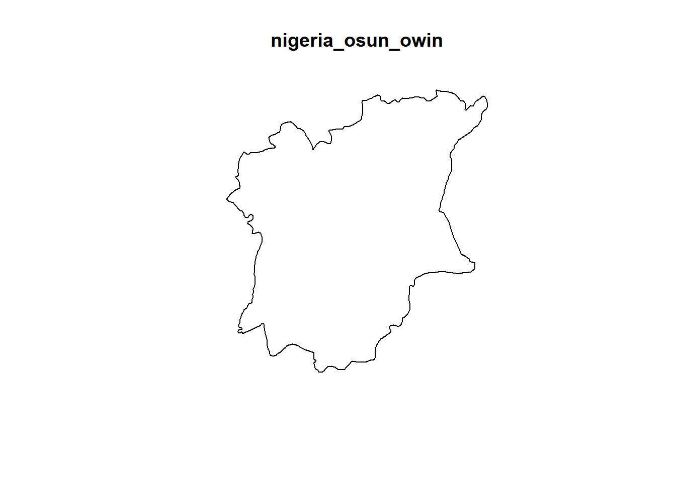
and summary() function of Base R.
summary(nigeria_osun_owin)Window: polygonal boundary
single connected closed polygon with 641 vertices
enclosing rectangle: [178398.73, 292278.89] x [329463.4, 452734.9] units
(113900 x 123300 units)
Window area = 8594710000 square units
Fraction of frame area: 0.6127.6 Combining Point Events Object and owin Object
In this last step of geospatial data wrangling, we will extract waterpoints events that are located within Osun using the code below
wpdx_ppp = wpdx_ppp[nigeria_osun_owin]
wpdx_func_ppp = wpdx_func_ppp[nigeria_osun_owin]
wpdx_nonfunc_ppp = wpdx_nonfunc_ppp[nigeria_osun_owin]The output object combined both the point and polygon feature in one ppp object class as shown below.
summary(wpdx_ppp)Planar point pattern: 5688 points
Average intensity 6.618021e-07 points per square unit
Coordinates are given to 2 decimal places
i.e. rounded to the nearest multiple of 0.01 units
Window: polygonal boundary
single connected closed polygon with 641 vertices
enclosing rectangle: [178398.73, 292278.89] x [329463.4, 452734.9] units
                     (113900 x 123300 units)
Window area = 8594710000 square units
Fraction of frame area: 0.612plot(wpdx_ppp)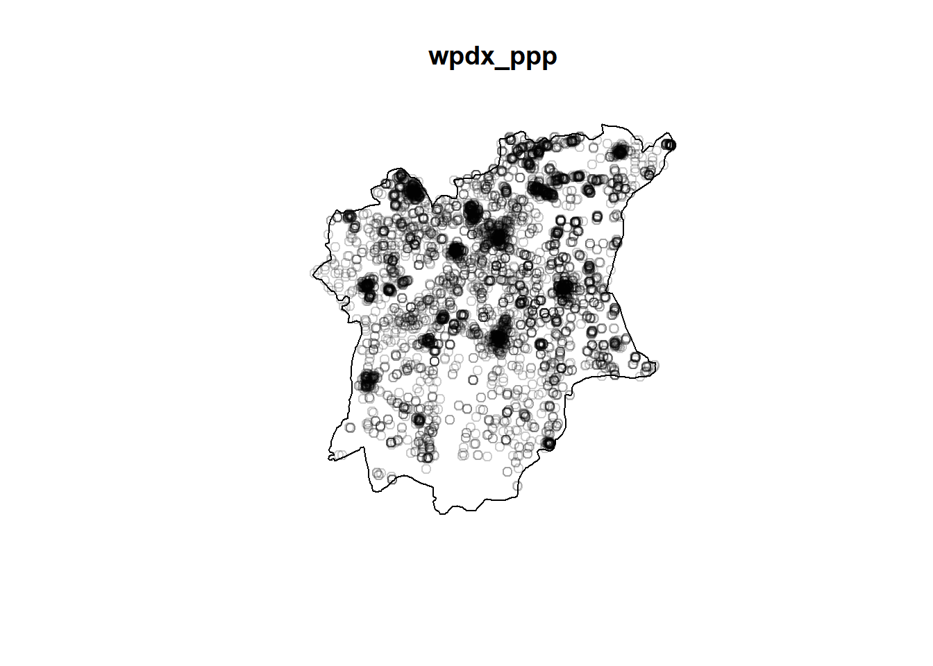
8 First-order Spatial Point Patterns Analysis
8.1 Kernel Density Estimation
8.1.1 Rescaling KDE Values
Using the rescale() function, we can convert the unit of measurement from metres to kilometres.
wpdx_ppp.km <- rescale(wpdx_ppp, 1000, "km")
wpdx_func_ppp.km <- rescale(wpdx_func_ppp, 1000, "km")
wpdx_nonfunc_ppp.km <- rescale(wpdx_nonfunc_ppp, 1000, "km")
8.1.2 Computing KDE by using Adaptive Bandwidth
The fixed bandwidth method is very sensitive to highly skewed distribution of spatial point patterns over geographical units (eg. urban vs rural). These helps us in the case of Osun where there are more urbanised and rural areas which we can see from the Openstreetmap above.
We can use density.adaptive() to derive adaptive kernel density estimation
kde_wpdx <- adaptive.density(wpdx_ppp.km, method = "kernel")
kde_wpdx_func <- adaptive.density(wpdx_func_ppp.km, method = "kernel")
kde_wpdx_nonfunc <- adaptive.density(wpdx_nonfunc_ppp.km, method = "kernel")
8.1.3 Converting KDE Output into Grid Object
The results are the same, but the conversion allows us to use it for mapping purposes.
gridded_kde_wpdx <- as.SpatialGridDataFrame.im(kde_wpdx)
gridded_kde_wpdx_func <- as.SpatialGridDataFrame.im(kde_wpdx_func)
gridded_kde_wpdx_nonfunc <- as.SpatialGridDataFrame.im(kde_wpdx_nonfunc)
8.1.3.1 Converting Gridded Output into Raster
Next, we will convert gridded kernel density objects into RasterLayer object using raster() of the raster object.
kde_wpdx_raster <- raster(gridded_kde_wpdx)
kde_wpdx_func_raster <- raster(gridded_kde_wpdx_func)
kde_wpdx_nonfunc_raster <- raster(gridded_kde_wpdx_nonfunc)
We can view the properties of kde_childcareSG_bw_raster RasterLayer
kde_wpdx_rasterclass : RasterLayer
dimensions : 128, 128, 16384 (nrow, ncol, ncell)
resolution : 0.8896887, 0.9630582 (x, y)
extent : 178.3987, 292.2789, 329.4634, 452.7349 (xmin, xmax, ymin, ymax)
crs : NA
source : memory
names : v
values : -1.256255e-15, 43.45513 (min, max)Note that the CRS property is NA.
8.1.3.2 Assigning Projection Systems
The code below will be used to include CRS information.
projection(kde_wpdx_raster) <- CRS("+init=EPSG:26391 +units=km")
projection(kde_wpdx_func_raster) <- CRS("+init=EPSG:26391 +units=km")
projection(kde_wpdx_nonfunc_raster) <- CRS("+init=EPSG:26391 +units=km")
kde_wpdx_raster
class : RasterLayer
dimensions : 128, 128, 16384 (nrow, ncol, ncell)
resolution : 0.8896887, 0.9630582 (x, y)
extent : 178.3987, 292.2789, 329.4634, 452.7349 (xmin, xmax, ymin, ymax)
crs : +proj=tmerc +lat_0=4 +lon_0=4.5 +k=0.99975 +x_0=230738.26 +y_0=0 +a=6378249.145 +rf=293.465 +units=km +no_defs
source : memory
names : v
values : -1.256255e-15, 43.45513 (min, max)Note that the CRS property has been included. We also include the units so that the map knows how to plot the raster based on the values later.
8.2 Visualising Output in tmap
We can finally display the raster using tmap
8.2.1 Kernel Density Estimate (KDE) of All Water Points
tmap_mode('view')
tm_basemap(server = "OpenStreetMap") +
tm_shape(kde_wpdx_raster) +
  tm_raster("v",
            title = "No. of Water Points",
            alpha = 0.6,
            palette = c("#eff3ff","#bdd7e7","#6baed6","#3182bd","#08519c"))
Note that the raster values are encoded explicitly onto the raster pixel using the values in the “v” field.
8.2.2 Kernel Density Estimate (KDE) of Functional and Non-Functional Water Points
tmap_mode('view')
func_map <- tm_basemap(server = "OpenStreetMap") +
              tm_shape(kde_wpdx_func_raster) +
                tm_raster("v",
                          title = "No. of Functional Water Points",
                          alpha = 0.6,
                          palette = c("#edf8e9","#c7e9c0","#a1d99b","#74c476","#31a354", "#006d2c"))

nonfunc_map <- tm_basemap(server = "OpenStreetMap") +
              tm_shape(kde_wpdx_nonfunc_raster) +
                tm_raster("v",
                          title = "No. of Non-Functional Water Points",
                          alpha = 0.6,
                          palette = c("#fee5d9","#fcae91","#fb6a4a","#de2d26","#a50f15"))


tmap_arrange(func_map, nonfunc_map)
By comparing the Functional and Non-Functional Water Points KDE Map, we can see that where places have a higher functional water points, it is usually the case to have similar numbers of non-functional water points.
Tip
KDE Plots makes it easier to see the density of features, a darker shade could imply that there are more occurences of events within that area. A point map would only show individual events and it is hard to pinpoint the density of points within the area if there are many events.
9 Second-order Spatial Point Patterns Analysis
There are four types of second-order spatial point pattern analysis that we can choose to select from to perform the analysis.
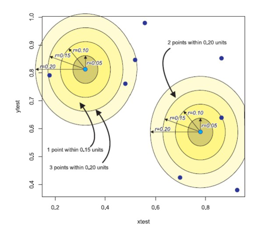
Figure of K-Function / L-Function Test from Prof Kam’s Lesson 04 Slides
L-Function test has been selected to perform the analysis as:
Accounts for edge correction for points that are slightly futher away from the main event but may still be useful
L-Function test is chosen over K-Function test as L-Function has been normalised to zero, making it easier to perform our analysis.
We will perform three L-Function Analysis to better understand the spatial correlation of:
- All water points in Osun, Nigeria
- Functional water points in Osun, Nigeria
- Non-functional water points in Osun, Nigeria
to better understand if there are any clustering, dispersion effects or if they are randomly distributed.
9.1 Analysing Spatial Point Process Using L-Function
In this section, we will use Lest() of spatstat to compute L Function estimation and also perform Monte Carlo simulation test using envelope() of spatstat.
9.1.1 All Water Points
9.1.1.1 Computing L Function Estimation
Using the code below, we run the L-Function estimation using the Ripley correlation to perform edge correction and plot the graph for our initial analysis.
L_wpdx = Lest(wpdx_ppp, correction = "Ripley")
plot(L_wpdx, . -r ~ r,
     ylab= "L(d)-r", xlab = "d(m)")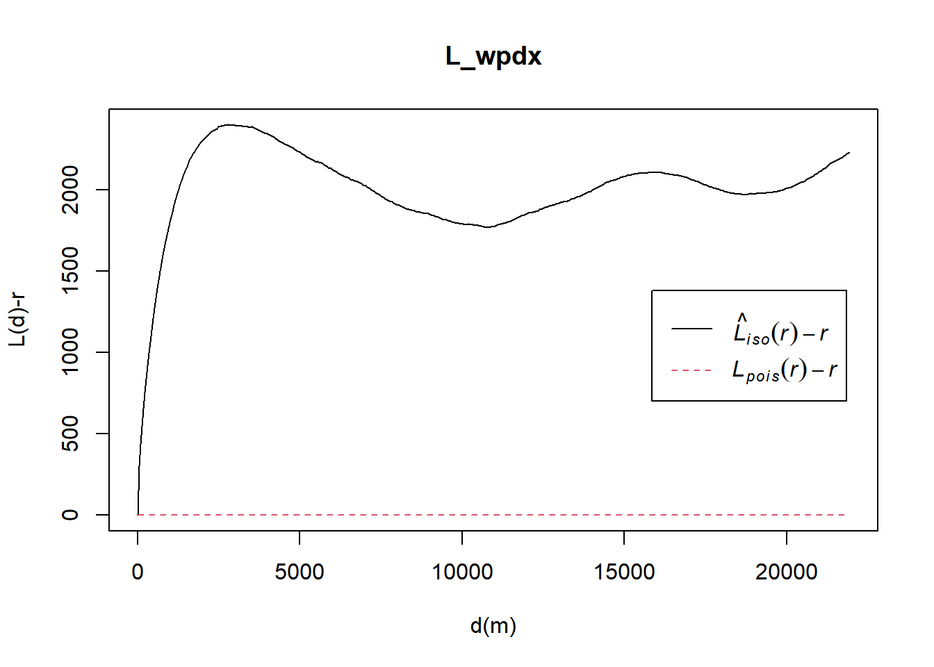
From the L function graph, we can see that there are signs of spatial clustering for all water points at all distances since Lobs(r) > Ltheo(r). However, we would require to perform a Monte Carlo simulation of events to statistically conclude if functional and non-functional water points are significant.
9.1.1.2 Performing Complete Spatial Randomness Test
To confirm the observed spatial patterns above, we will conduct a hypothesis test. The hypothesis and test are shown below:
Ho = The distribution of water points in Osun, Nigeria are randomly distributed.
H1= The distribution of water points in Osun, Nigeria are not randomly distributed.
The null hypothesis will be rejected if p-value if smaller than alpha value of 0.05 (confidence interval of 95%).
The code chunk below is used to perform the hypothesis testing.
Note
We have set to not evaluate the simulation on render. The code below is to run the simulation, save it to an RDS file so it can be imported on render to be plotted as a graph
L_wpdx.csr <- envelope(wpdx_ppp, Lest, nsim = 39, rank = 1, glocal=TRUE)#saveRDS(L_wpdx.csr, "Take-Home_Ex01/data/rds/L_wpdx_csr.rds")L_wpdx.csr <- readRDS("Take-Home_Ex01/data/rds/L_wpdx_csr.rds")plot(L_wpdx.csr, . - r ~ r, xlab="d", ylab="L(d)-r")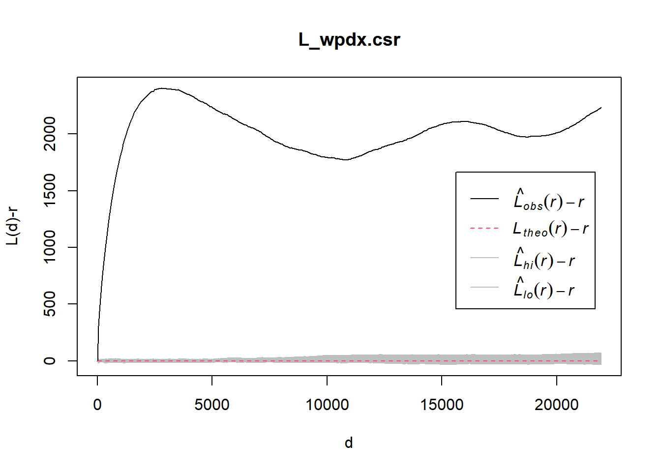
From the graph above, for all distances, L(r) - r for water points in Osun, Nigeria are above 0 and lies outside of the lower and higher confidence interval envelope.
Hence, from this observation, since L(r) - r is outside the higher confidence interval envelope, we havesufficient evidence to reject the null hypothesis that The distribution of water points in Osun, Nigeria are randomly distributed.
Since L(r) - r > 0, it indicates that the observed distribution is geographically concentrated.
9.1.2 Functional Water Points
9.1.2.1 Computing L Function Estimation
Using the code below, we run the L-Function estimation using the Ripley correlation to perform edge correction and plot the graph for our initial analysis.
L_func = Lest(wpdx_func_ppp, correction = "Ripley")
plot(L_func, . -r ~ r,
     ylab= "L(d)-r", xlab = "d(m)")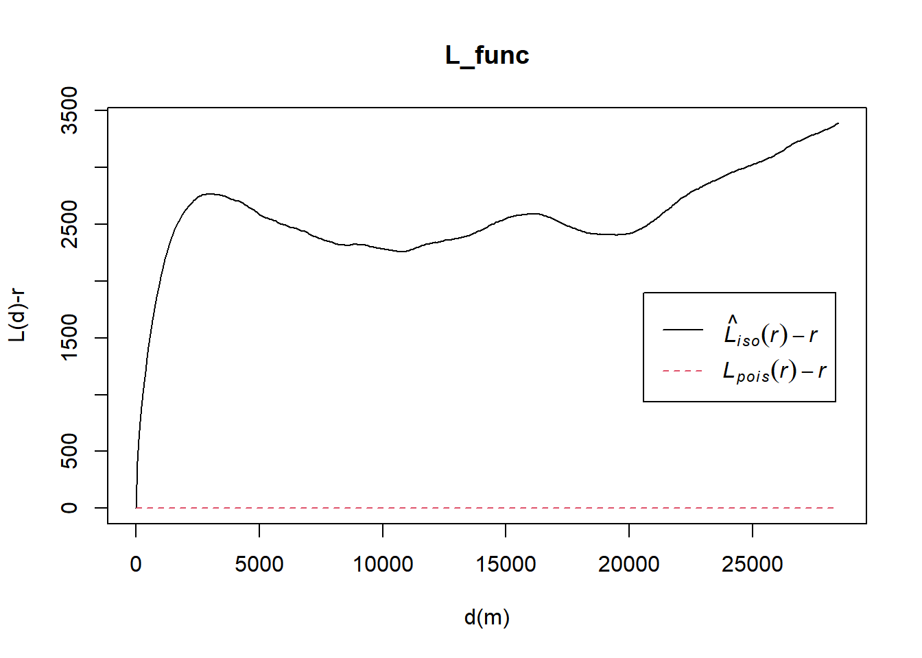
From the L function graph, we can see that there are signs of spatial clustering for all water points at all distances since Lobs(r) > Ltheo(r). However, we would require to perform a Monte Carlo simulation of events to statistically conclude if functional water points are significant.
9.1.2.2 Performing Complete Spatial Randomness Test
To confirm the observed spatial patterns above, we will conduct a hypothesis test. The hypothesis and test are shown below:
Ho = The distribution of functional water points in Osun, Nigeria are randomly distributed.
H1= The distribution of functional water points in Osun, Nigeria are not randomly distributed.
The null hypothesis will be rejected if p-value if smaller than alpha value of 0.05 (confidence interval of 95%).
The code chunk below is used to perform the hypothesis testing.
Note
We have set to not evaluate the simulation on render. The code below is to run the simulation, save it to an RDS file so it can be imported on render to be plotted as a graph
L_func.csr <- envelope(wpdx_func_ppp, Lest, nsim = 39, rank = 1, glocal=TRUE)#saveRDS(L_func.csr, "Take-Home_Ex01/data/rds/L_func_csr.rds")L_func.csr <- readRDS("Take-Home_Ex01/data/rds/L_func_csr.rds")plot(L_func.csr, . - r ~ r, xlab="d", ylab="L(d)-r")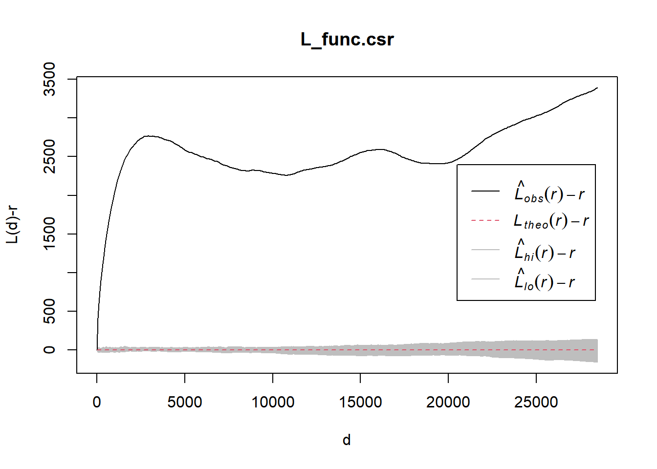
From the graph above, for all distances, L(r) - r for functional water points in Osun, Nigeria are above 0 and lies outside of the lower and higher confidence interval envelope.
Hence, from this observation, since L(r) - r is outside the higher confidence interval envelope, we have sufficient evidence to reject the null hypothesis that The distribution of functional water points in Osun, Nigeria are randomly distributed.
Since L(r) - r > 0, it indicates that the observed distribution is geographically concentrated.
9.1.3 Non-Functional Water Points
9.1.3.1 Computing L Function Estimation
Using the code below, we run the L-Function estimation using the Ripley correlation to perform edge correction and plot the graph for our initial analysis.
L_nonfunc = Lest(wpdx_nonfunc_ppp, correction = "Ripley")
plot(L_nonfunc, . -r ~ r,
     ylab= "L(d)-r", xlab = "d(m)")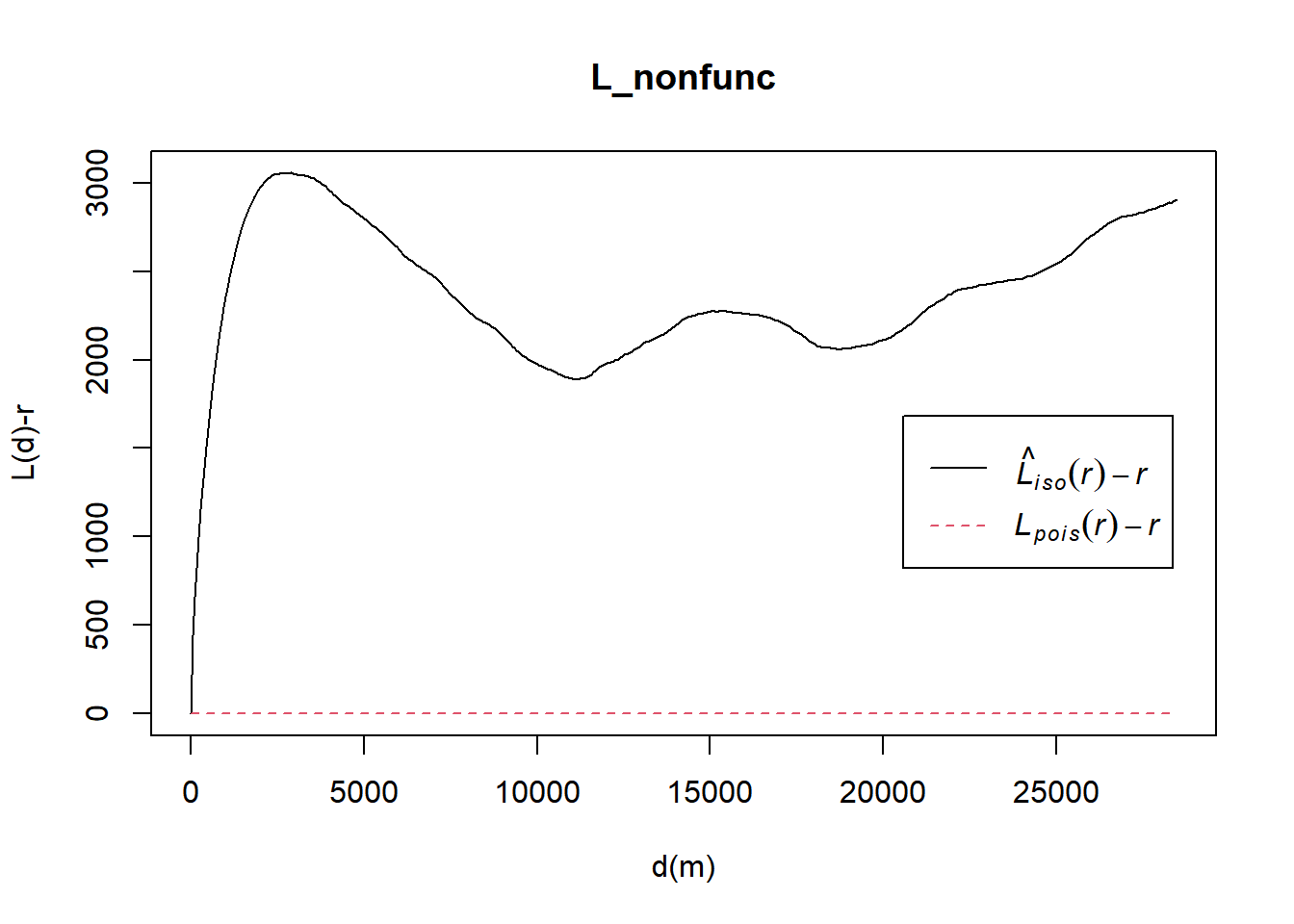
From the L function graph, we can see that there are signs of spatial clustering for non-functional water points at all distances since Lobs(r) > Ltheo(r). However, we would require to perform a Monte Carlo simulation of events to statistically conclude if non-functional water points are significant.
9.1.3.2 Performing Complete Spatial Randomness Test
To confirm the observed spatial patterns above, we will conduct a hypothesis test. The hypothesis and test are shown below:
Ho = The distribution of non-functional water points in Osun, Nigeria are randomly distributed.
H1= The distribution of non-functional water points in Osun, Nigeria are not randomly distributed.
The null hypothesis will be rejected if p-value if smaller than alpha value of 0.05 (confidence interval of 95%).
The code chunk below is used to perform the hypothesis testing.
Note
We have set to not evaluate the simulation on render. The code below is to run the simulation, save it to an RDS file so it can be imported on render to be plotted as a graph
L_nonfunc.csr <- envelope(wpdx_nonfunc_ppp, Lest, nsim = 39, rank = 1, glocal=TRUE)#saveRDS(L_ck.csr, "Take-Home_Ex01/data/rds/L_nonfunc.rds")L_nonfunc.csr <- readRDS("Take-Home_Ex01/data/rds/L_nonfunc.rds")plot(L_nonfunc.csr, . - r ~ r, xlab="d", ylab="L(d)-r")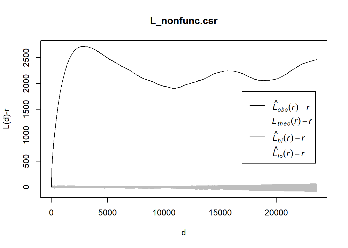
From the graph above, for all distances, L(r) - r for non-functional water points in Osun, Nigeria are above 0 and lies outside of the lower and higher confidence interval envelope.
Hence, from this observation, since L(r) - r is outside the higher confidence interval envelope, we have sufficient evidence to reject the null hypothesis that The distribution of non-functional water points in Osun, Nigeria are randomly distributed.
Since L(r) - r > 0, it indicates that the observed non-functional water point distribution is geographically concentrated.
10 Conclusion
From the KDE Plots, we can see clearly, a trend where functional and non-functional water points will be denser in denser urban areas which are denoted by areas with a denser network of roads.
Utilising spatial point patterns analysis with L-function estimation and Monte Carlo Test, we can confirm that the water points (a. all water points, b. functional water points, c. non-functional water points) in its own groups are not randomly distributed and are in fact geographically concentrated, which we could see on the point patterns tmap and KDE plot that we have plotted earlier.
11 References
- Prof Kam’s Hands-on Exercises, In-Class Exercises and Lecture Materials
- Sylvester O, E., Olujimi F, O. and Sunday A, O. (2018) “On the determination of NTM and UTM positions from post processing of static DGPS observations on the Nigeria Minna Datum,” International Journal of Engineering Research and Advanced Technology, 4(10), pp. 10–24. Available at: https://doi.org/10.31695/ijerat.2018.3332.